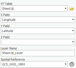
...

The Geoprocessing pane should open on the right in a new tab overlaying the Catalog pane. In the 'Make XY Event Layer' tool, notice that 'XY Table' is already set to the Sheet1$ table, since that was the table used to open the tool.

...

Notice in the ‘Spatial Reference’ drop-down menu, it defaults to GCS_WGS_1984, which is the most commonly used geographic coordinate system for mapping latitude and longitude and happens to be the correct one to select in this case.

1. Ensure that your window matches that 'Copy Features' tool parameters match those shown below and click OK.
   
   
   
   
2. Click Run.

...

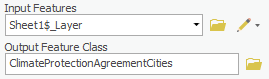
In the Geoprocessing pane, in the 'Copy Features' tool, notice that for 'Input Features' Sheet1$_Layer is already selected, since that was the table used to open the tool.

1. For ‘Output Feature Class’, rename the feature class from Sheet1_Features_CopyFeatures to “ClimateProtectionAgreementCities”.
2. Ensure your Geoprocessing pane appears as shown below and click Run.
   
   Image Added

Since you are now using have a permanent feature class, you may remove your temporary Sheet1$ layer and the corresponding Excel table.

1. Right-click the Sheet1$_Layer layer and select Remove.
2. Right-click the Sheet1$ standalone table and select Remove.

If you’d like to get a better view of your points, use the navigation navigate tools on the Map tab to zoom in to the continental United States. You have successfully mapped point locations using XY coordinates.

Bonus Exercise: Spatial Join

At this point, all of the cities appear on the map, but there are many urban areas that are so densely covered with overlapping points that it becomes difficult to tell exactly how many points there are and to see the underlying data, such as city and state names. In addition, while you can see the spatial distribution of the points, you are not provided with any sort of useful summary of the data. Performing a spatial join will allow you to discover how many participating cities are located in each state, or even county.

1. At the bottom of the Geoprocessing pane, click the Catalog pane tab.
2. Expand the Databases folder.
3. Expand the XY geodatabase to expand its contents.

Notice that the ClimateProtectionAgreementCities feature class you just exported is now contained in this geodatabase.

...

1. In the Contents pane, right-click the US_States layer and select Attribute Table.
2. Scroll to the right and browse through all of the attributesattribute fields.

The goal of performing a spatial join is to add a numeric field to the end of this attribute table that tells you how many participating cities are contained within each state.

1. Close the US_States table view.
2. In the Contents pane, right-click the US_States layer and selectJoins and Relates > Spatial Join.

The Spatial Join tool will open within the Geoprocessing pane. For 'Target Features', the US_States layer is already selected, since that is the layer from which you launched the tool.

1. For ‘Join Features’, use the For the ‘Join Features’ drop-down menu , to select the ClimateProtectionAgreementCities layer..
2. For the ‘Output Feature Class’, rename the feature class from US_States_SpatialJoin to “US_States_WithCityCounts”.

The 'Field Map of Join Features' describes how the features will be summarized as they are joined. The first half of the list of fields displays the attributes of the states layer, ending with the Shape_Area field. The second half of the list of fields, beginning with the Latitude field, displays the attributes of the cities layer. A count field indicating how many city points intersect with each state will automatically be provided. Since many cities will be appended to each state, it does not make sense to generate summary statistics about the city fields, because variables like latitude, longitude, and name cannot be averaged. By default, the table would output only the attributes of the first city encountered within each state, which could be very misleading. Therefore, you will remove all the city attributes from the output fields.

Hypothetically, if Notice that by default, each polygon will be given a count field showing how many points fall inside it, so you do not need to pick an additional statistic.  If, for example, your cities layer contained an attribute listing the population of each participating city, then, when performing the spatial join, you could check the ‘Sum’ statistic use the Sum Merge Rule on the population field to calculate the total population residing in participating cities in each state and then calculate what percentage of the state’s total population reside in these participating cities. In this case, you do not have such population data available, so you will stick with the default Join Count attribute..

1. Within 'Output Fields', click the Latitude field.
2. Hold down Shift and click the last State field, so that all four city fields (Latitude, Longitude, City, State) are selected.
   
3. Right-click the selected State field and select Remove.
4. Click For the ‘Output Feature Class’ drop-down menu, select the Browse button next to it, ensure it is within the XYData.gdb, and name it “US_States_WithCityCounts”. Click Save and click Run.

The new layer should appear at the top of your Contents pane. 

1. At the top of the Contents pane, right-click the US_States_WithCityCounts layer and select Attribute Table.
2. Notice the third column contains the newly-added Join_Count field.  This field tells you how many participating cities are contained within each state.
3. Close the US_States_WithCityCounts table view.

Since the new layer contains all of the same information as the old US_States layer, plus the new Join_Count field, you no longer need the US_States layer.

1. In the Contents pane, right-click the US_States layer and select Remove.
2. Right-click the US_States_WithCityCounts layer and select Symbology.
3. In the Symbology pane, in use the Symbology drop-down menu , to select Graduated Colors.
4. In For 'Field’, use the ‘Fields’ drop-down menu , to select the Join_Count field.

You can now easily tell which states have the largest number of participating cities, though this display does not take into consideration things such as city density and population density or the percentage of the total state population participating.

1. Above the ribbon, on the Quick Access toolbar, click the Save button.
   
   Image AddedOn the toolbar at the top of the Map Window, click Save.
   
   
2. Close ArcGIS Pro.

Optional Exercise: Converting Addresses to XY Coordinates

If all of your data already comes with a list of the latitudes and longitudes of the points you’d like to map, then you are ready to go straight into ArcMapArcGIS Pro, but what if you have a list of cities or addresses that you’d like to map, but you don’t know their corresponding coordinates? This section will show you one automated method of generating such coordinates based on address locations.

...

1. On the Desktop, double-click the XY folder.
2. Double-click Cities_ClimateProtectionAgreementMayors.xls to open the file with Excel.

Notice this file is identical to the worksheet you used earlier to map the participating city locations, except that it is missing the latitude and longitude information. In such an instance where you would like to map these cities, you would first have to obtain their coordinates, so you will use an online geocoder. There are many online geocoders, but the one you will be using in this course is called GPSVisualizer. For your future reference, a list of geocoders is maintained by the University of Southern California GIS Research Laboratory at httpsTexas A&M University GeoServices at http://webgisgeoservices.usctamu.edu/Services/Geocode/AboutOtherGeocoders/GeocoderList.aspx.

1. Minimize or Restore Down Excel.
2. On the Desktop, double-click the Mozilla Firefox Google Chrome icon.
3. In the location bar, type “gpsvisualizer.com” and press Enter.
4. At the top of the ‘GPSVisualizer’ window, click Geocode an addressaddresses.
   

...

1. 
   Image Added

Here, you will see several options for geocoding addresses. Option 2 allows you to geocode multiple addresses and should be used for standard street addresses, but Option 3 allows you to geocode simple locations and is recommended if you are mapping data such as ZIP codes, cities, or states. Since your data table only contains city names, you will use option 3.

1. Under ‘3. Geocode simple tabular data’, click the link to the text/GPX conversion utility.
2. Return to the Excel spreadsheet.
3. Click the Select All button in the top left corner of the spreadsheet.
   
   Image Added
   
   
4. In the Home tab, click Copy.
5. Return to GPSVisualizer.
6. In the ‘Or paste your data here:’ box, delete all existing text.
7. Right-click in the ‘Or paste your data here:’ box and select Paste to copy in the city data from your Excel worksheet.
8. Click Convert.

...

1. Towards the top of the window, right-click the link that says following link and select Save Link As…link as….  (Yours will have a different download number than shown below.)
   
   Image Added
   
   
2. Double-click the XY folder.
3. Rename For 'File name:' rename your file “LatLongMayors” “LatLongMayors” and click Save.
4. Return to Excel.
5. At the bottom of the worksheet, click the Insert Worksheet button.
   
   
6. Click the Data tab.
7. Under the ‘Get External Data’ section, click From Text.
8. Navigate to select your saved LatLongMayors text file (Desktop > XYTutorialData > LatLongMayors) and click Import.
9. In the ‘Text ImportWizard’ window, ensure that Delimited is selected and click Next >.

...