...
13. Ensure your ‘Project’ window appears as shown below and click Run.

14. Close Geoprocessing Pane.
...
20. On the ‘Coordinate System’ tab toolbar, click the Add Coordinate System button and select Import….

21. Double-click the HyrdologyLab geodatabase.
...
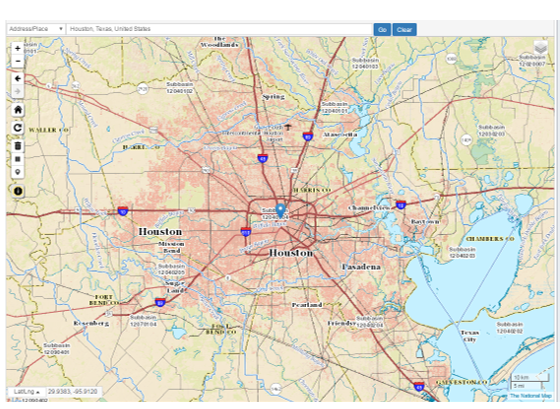
After zooming into Houston, you can see the blue boundaries of the individual subbasins and each subbasin is labeled with its HUC-8 number on the map.
- Near the center of the map, click within Subbasin 12040104 to select it.

Notice that just above the map, your search is now constrained to Polygon: huc8 12040104.
- At the top of the left side bar, click Find Products.

- Under Available Products, to the right of Elevation Products (3DEP), click results.
...
You are now provided with a listing of all the DEM tiles covering the area of Subbasin 12040104.

10. In turn, click Download for USGS NED n30w096, n30w095, and n31w096.

11. Navigate to the location where the three zipped folders have been downloaded.
...
10. Ensure your ‘Mosaic To New Raster’ appears as shown below and click Run.

The mosaic may take a couple minutes to process. When it is complete, notice there are no longer visual seams between the tiles in the mosaicked raster. Now that you have a single mosaic, you no longer need the three originals tiles.
...
- Leave ‘Output Cell Size’ blank, but type “300” for the ‘X’ and ‘Y’. Make sure that your screen is the same as the screenshot below. Click Run.

Remember that the data frame was already displaying all layers in State Plane Texas South Central, so you should not notice much of a difference between the two layers, other than that the cell size has increased, meaning the resolution has decreased.
...
- For ‘Output Raster Dataset’, rename the raster from “DEMStatePlane_Clip” to “DEMSubbasin”.
- Ensure your ‘Clip’ window appears exactly as shown below and click Run.

- Remove the DEMStatePlane layer from the Table of Contents.
- Turn off the Watersheds_StatePlane layer to view the DEMSubbasin layer.
...
- In Geoprocessing pane, click the Spatial Analyst Tools toolbox à Map Algebra toolset à Raster Calculator tool.
- In the list of ‘Layers and variables’, double-click the DEMSubbasin layer.
- In the calculator, double-click the * button.
- In the equation box, type “3.281”, which is the conversion factor from meters to feet.
- For ‘Output raster’, rename the raster from “rastercalc” to “DEMft”.
- Ensure your ‘Raster Calculator’ window appears as shown below and click Run.

Visually, the meters and feet layers should be identical, but if you look at the layers in the Table of Contents, you will notice that the original layer goes from elevations of -8 to 62 meters and the newly calculated layer goes from elevations of -26 to 204 feet.
...
- Again, go back to the Raster Calculator tool. Delete the previous expression.
- In the list of ‘Layers and variables’, double-click the DEMft layer.
- In the calculator, double-click the <= button.
- In the equation box, type “15”.
- For ‘Output raster’, rename the raster from “demft_raster” to “Flood15ft”.
- Ensure your ‘Raster Calculator’ window appears as shown below and click Run.

- Close Geoprocessing pane.
- Right-click the Flood15ft layer. Click Symbology.
- In the table of values, right-click the 0 value and click Remove.

10. Click the rectangle symbol to the left of the 1 value and select Blue.

11. Save your map document.
...
Create an 8.5 x 11 layout showing the DEM clipped to the subbasin with areas less than or equal to 15 feet in elevation highlighted.

Symbolizing raster files
...
- Click the Insert menu and select New Map….
- Double-click “Map1” in the contents pane and type “Lab2Topo” as name. Click Save.
- Expand Databases in the Catalog pane. Click HydrologyLab.gdb.
- Drag the DEMft and Watersheds_Stateplane layers into the map display.
- Turn off the Watersheds_Stateplane layer.
- Right-click DEMft layer and click the Symbology.
- Scroll down the ‘Color Ramp’ drop-down menu and select the rainbow ramp.

Patterns within the data are now easier to see, especially at the lower elevations.
...
- For ‘Z factor’, leave the default value of 1.
- Ensure your ‘Contour’ window appears as shown below and click Run.

- Turn off the DEMft layer to better see the contours.
...
13. Use the ‘Color Ramp’ drop-down menu. Check Show All and select one of the few graduated color ramps as shown below.

Now you can tell which contours are highest and lowest.
...
- For ‘Z factor’, type “20”.
- Ensure your ‘Hillshade’ window appears as shown and click Run.

Typically hillshades are shown beneath transparent layers conveying other information, just to give the map a realistic appearance.
...