Page History

...

1. Using a web browser, search for "h-gac gis" and select the result as shown below or go directly to: http://www.h-gac.com/gis-applications-and-data/datasets.aspx
   
   
   
   
2. Under the 'Dataset Categories' section, click the Hydrologic button to filter the results by subject.
   
   Image Modified
   
   
3. Under the 'Datasets' section, click Major Rivers.
   
   Image Modified
   
   
4. Click Download Dataset in the pop-up window.
5. Click the blue Download button in the top right corner of the new window.

...

1. From the Windows Taskbar, click the blue globe icon to launch ArcGIS Pro.
   
   
   
   
2. When ArcGIS Pro opens, under the 'Create a new project' section on the right side of the screen, click the Blank project template.
   
   Image Modified
   
   
3. In the 'Create a New Project' window, for the 'Name' input, type "Intro_Part2".
4. For 'Location', click the yellow Browse... button to the right.
5. In the 'Select a folder to store the project.' window, click Computer in the left column and click Desktop in the right column and click OK.
   
   Image Modified
   
   
6. In the 'Create a New Project' Window, click OK.
7. Maximize the ArcGIS Pro application window.

...

1. In the Catalog pane, right-click Folders and select Add Folder Connection.
2. In the left column click This PC. In the right column, click Downloads and click OK.
3. In the Catalog pane, expand Downloads.
4. Fully expand all folders and geodatabases in the Downloads folder.
5. We will repeat the above process to connect to a folder containing a sample of NHGIS data. In the Catalog pane, right-click Folders and select Add Folder Connection.
6. In the left column click This PC. In the right column, click gisdata (\\file-rnas.rice.edu)(R) > Short_Courses_HIST207 > HIST207_GDC2 > NHGIS_Data and click OK.
7. In the Catalog pane, expand NHGIS_Data.
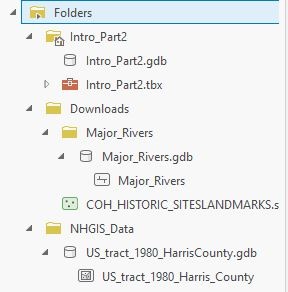
8. Your 'Folders' directory should look like the below.
   Image Removed
   Image Added

Importing and Exporting Data in the Project Geodatabase

...

1. In the Catalog pane, click the US_tract_1980_Harris_County geodatabase feature class located in the NHGIS folder and drag-and-drop it into the Intro_Part2.gdb. A progress bar will appear that reads 'Copying...' Once it is complete, you will see a copy of US_tract_1980_Harris_County inside the Intro_Part2.gdb as shown below.
   
   
   
   
2. Repeat the above step to drag-and-drop Major_Rivers from the Major_Rivers.gdb into the Intro_Part2.gdb. 
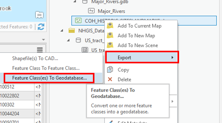
3. COH_HISTORIC_SITESLANDMARKS is a Shapefile feature class, so it requires a different method to be imported into the Project Geodatabase. In the Catalog pane, right-click on COH_HISTORIC_SITESLANDMARKS.shp and select Export > Feature class(es) to geodatabase.
   
   Image Modified
   
   
4. In the Geoprocessing pane, accept default settings as shown below and click Run. 
   
   Image Modified
   
   
5. In the Catalog pane, right-click on Intro_Part2.gdb and select Refresh. 
   
   Image Modified
   
   
6. Your Project Geodatabase should now contain three Geodatabase feature classes: COH_HISTORIC_SITESLANDMARKS, Major_Rivers, and US_tract_1980_Harris_County.
   
   
   
   
7. In the Catalog pane, in the Folders section, right-click on Downloads and select Remove.
   
   
   
   
8. Repeat Step 7 to remove the connection to the NHGIS folder.

...

1. On the ribbon, click the Insert tab.
2. In the Project group, click the New Map button.
   
   
   
   
3. In the Catalog pane, right-click the US_tract_1980_Harris_County feature class and select Add To Current Map.
4. Above the ribbon, on the Quick Access toolbar, click the Save button.

...

1. In the Contents pane, right-click the US_tract_1980_Harris_County layer name and select Symbology.
2. In the Symbology pane, click the primary drop-down menu and select Graduated Colors.
   
   
   
   
3. Use the 'Field' drop-down menu to select the AV0AA1980 field. NHGIS data downloads include a read-me file that defines the codes for each field (column). AV0AA1980 stores the number of people within each census tract for the year 1980.
   
   The Map View now displays a choropleth map, where the darker colors represent higher numbers of people. In studying the map, it appears as if there is no discernible pattern to population numbers. While this is true according to raw counts per census tract, there could be differences in the census tracts that are unaccounted for in this symbology. Now you will try normalizing by the area of the census tracts.
   
   
4. Use the 'Normalization' drop-down menu to scroll to the bottom and select the last Shape_Area field. 
   
   Note: the projection of the census layer is GCS WGS 1984. Therefore, the layer is unprojected and the coordinates are stored in angular units of decimal degrees. Therefore, the Shape_Area field is displaying square decimal degrees and the map is displaying number of people per square decimal degree. This is a somewhat incomprehensible unit, however, the values are still proportional to how they would be in a different unit and the relative coloring on the map remains correct. Notice that according to the density of population count, the greatest amount of people appear to be inside the major loops.
   
   
5. On the lower half of the Symbology pane, click the Histogram tab.
   Image Removed
   Image Added
   
   
6. Use the 'Method" drop-down menu to select Equal Interval.
7. Use the 'Method" drop-down menu to select Quantile.
8. Use the 'Classes' drop-down menu to select 20.
9. Use the 'Classes' drop-down menu to select 2.
10. Use the 'Color Scheme' drop-down menu to select a different color scheme of your choice.

...