Page History

...

1. On the catalog pane, expand Databases and HydrologyLab.gdb file.
2. Drag the Watersheds feature class into the Map Display.
3. In the Table of Contents, double-click the Watersheds layer.
4. In the ‘Layer Properties’ window, click the Source tab and expand Spatial Reference.
   
   Notice that the layer is in a geographic coordinate system called GCS_North_American_1983. Because the data has a geographic coordinate system, the coordinates are stored in degrees, which indicate the three-dimensional spherical location of the data. Though the data itself is stored in a geographic coordinate system, your computer monitor is flat, so, though no projection has been defined, the data must be displayed in a particular projection. Whenever ArcMap displays data in a geographic coordinate system, it uses a Plate_Carrée projection, where one degree of latitude by one degree of longitude is represented as a square, rather than a curved trapezoid. This projection results in increasing stretching in the east-west direction, the farther north or south from the equator you are mapping.
   
   
5. Close the ‘Layer Properties’ window.
   
   Working with geographic coordinate systems is fine for creating purely visual maps, as you did in Lab 1 (though the visual distortion can be disorienting and misleading), but in this lab, you will be calculating areas, distances, and overlaps between features. Such calculations require the three-dimensional coordinates to be projected down onto a two-dimensional plane, so that the coordinates are stored in linear units, such as feet or meters, rather than degrees. In order to facilitate measurements of distance and area, you will now project the Watersheds layer into the State Plane Texas South Central projection which is best suited to mapping the greater Houston region.
   
   
6. In the Analysis tab, click Tools.
7. Under Toolboxes, double-click the Data Management Tools toolbox → Projections and Transformations toolset → Project tool.
8. For ‘Input Dataset or Feature Class’, use the drop-down menu to select Watersheds layer.
   Note that the input coordinate system is GCS_North_American_1983
9. , as you previously determined and cannot be changed.
   Also notice that the output dataset defaults to your ElevationRainfall geodatabase.
   For ‘Output Dataset or Feature Class’, rename “Watersheds_Project” to “Watersheds_StatePlane”, since that is the name of the projection you will be using.
10. Next to the ‘Output Coordinate System’ box, click the Set Coordinate System button.
11. Double-click Projected Coordinate Systems → State Plane → NAD 1983 (2011) (US Feet).
12. Select NAD 1983 StatePlane Texas S Central FIPS 4204 (US Feet) and click OK.
    
    Because both the input and output coordinate systems are based on the NAD 1983 geographic coordinate system, no geographic transformation is required.
    
    
13. Ensure your ‘Project’ window appears as shown below and click Run.
    
14. Close Geoprocessing Pane.
    
    Now that you have the correctly projected layer, you no longer need the original NAD 1983 layer.
    
    
15. Right-click the Watersheds layer and select Remove.
16. Double-click the new Watersheds_StatePlane layer.
    
    Notice that the layer is now in a projected coordinate system, NAD_1983_StatePlane_Texas_South_Central_FIPS_4204_Feet.
    
    
17. Close the ‘Layer Properties’ window.
    

    You may have noticed that the visual appearance of the watersheds did not change in your Map Display, even though you projected them. That is because the data frame takes on the projection of the first layer added to it. Since you first added the original unprojected Watersheds layer into the data frame, which was in NAD 1983, the data frame displays the data in NAD 1983 (or Plate_Carrée). Currently, the projected Watersheds_StatePlane layer is being projected-on-the-fly back into NAD 1983 for visual purposes, so that the two layers are properly aligned in space.

    Move the cursor around the screen and notice that the coordinates in the bottom right corner of the Map Display are shown in decimal degrees. This is another clue that the data frame is still using a geographic coordinate system; however, you would like the data frame to display data using the local Houston projection.
    
    

18. At the top of the Table of Contents, right-click the Lab 2 map title and click Properties.

19. Click the Coordinate System tab.
    
    While you could search for or navigate to the State Plane Texas South Central coordinate system, as you did before, in this case, you know that the same coordinate system is already used by the Watersheds_StatePlane layer. In such an instance, it is often easier to import the coordinate system from another known layer, especially if you are not familiar with the hierarchy of the coordinate system folders
    
    

20. On the ‘Coordinate System’ tab toolbar, click the Add Coordinate System button and select Import….
    

21. Double-click the HyrdologyLab geodatabase.
22. Select the Watersheds_StatePlane feature class and click Add.
    
    Notice that the familiar State Plane Texas South Central projection is now listed.
    
    
23. Click OK.
    
    Notice that the watershed boundaries are now more compact in the east-west direction, as expected, because the local projection results in less distortion than the Plate Carrée projection used to represent geographic coordinate systems.
    
    

...

1. In a web browser, go to https://viewer.nationalmap.gov/basic/.
   
   First you will select the data products you are interested in viewing and downloading.
   
   
2. On the left side bar, check the Elevation Products (3DEP) section to expand it.
3. Within the Product Search Filter, check 1/3 arc-second DEM for the subcategory and select ArcGrid for the File Format.
4. On the left side bar, scroll below the Elevation Products section and check the Hydrography (NHDPlus HR, NHD, WBD) section to expand it.
5. Within the Product Search Filter, select National Hydrography Dataset (NHD) for the subcategory, select HU-8 Subbasin for the Data Extent and select FileGDB10.1 for the File Format.
   
   Now you constrain your downloads to your area of interest.
   
   
6. In the search bar just above the map on the right, type “Houston” and click Go.
   
   After zooming into Houston, you can see the blue boundaries of the individual subbasins and each subbasin is labeled with its HUC-8 number on the map.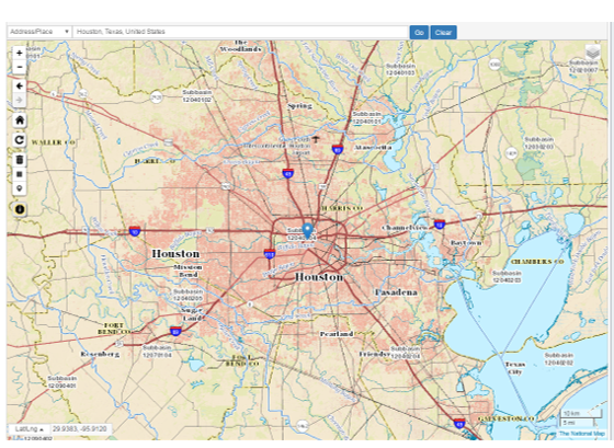
   
7. Near the center of the map, click within Subbasin 12040104 to select it.
   
   Notice that just above the map, your search is now constrained to Polygon: huc8 12040104.
   
   
8. At the top of the left side bar, click Find Products.
   
9. Under Available Products, to the right of Elevation Products (3DEP), click results.
   
   You are now provided with a listing of all the DEM tiles covering the area of Subbasin 12040104.
   
10. In turn, click Download for USGS NED n30w096, n30w095, and n31w096.
    
11. Navigate to the location where the three zipped folders have been downloaded.
12. Select and copy all three zipped folders.
13. Using Windows Explorer, navigate to your HydrologyLab folder.
14. Paste all three zipped folders directly inside your HydrologyLab folder. Do NOT paste them inside the .gdb geodatabase.
15. Select all three zipped folders.
16. Right-click any of the three selected folders and select 7-Zip → Extract to “*\”, which will create one unzipped folder for the contents of each zipped folder.
17. Return to ArcGIS Pro.
    
    Since you just added new files to your folder, you will need to refresh it in order for them to appear in ArcCatalogthe Catalog pane.
    
    
18. Click the Project tab on the Catalog pane.
19. Right-click your HydrologyLab folder and select Refresh.
20. Expand n30w095 and the other folders to preview their contents.
    
    Each raster file with a name such as grdn30w095_13 corresponds to a 1x1 degree tile. The file name contains “grd” for grid, followed by the latitude and longitude of the top left corner of the tile.

...

1. Close the ‘Layer Properties’ window.
2. Open Tools. Click Toolboxes on the geoprocessing pane.
3. In the Data Management Tools toolbox, click the Raster toolset → Raster Dataset toolset → Mosaic to New Raster tool.
4. For ‘Input Rasters’, select the three 1x1 degree raster layers.
5. For ‘Output Location’, click the Browse button.
6. Select the Lab1 HydrologyLab geodatabase and click Add.
7. For ‘Raster Dataset Name with Extension’, type “DEMMosaic”.
8. Use the ‘Pixel Type’ drop-down menu to select 32 bit float, since that was the same type stored in the original rasters.
9. For ‘Number of Bands’, type “1”. (The text appears on the right side of the field.)
10. Ensure your ‘Mosaic To New Raster’ appears as shown below and click Run.
    
    The mosaic may take a couple minutes to process. When it is complete, notice there are no longer visual seams between the tiles in the mosaicked raster. Now that you have a single mosaic, you no longer need the three originals tiles.
    
    
11. Remove all three original raster files from the Table of Contents.

...

1. In the Geoprocessing pane, click Data Management Tools -> Projections and Transformations toolset -> the Raster toolset à Project Raster tool.
2. For ‘Input Raster’, select in the DEMMosaic layer in the drop-down menu.
3. For ‘Output Raster Dataset’, rename the raster from “DEMMosaic_ProjectRaster” to “DEMStatePlane”
4. For ‘Output Coordinate System’, select Watersheds_Stateplane.

...

1. In ArcToolbox, back in the Raster toolset, double-click the Raster Processing toolset à and click the Clip (Data Management) tool.
2. For ‘Input Raster’, drag in the DEMStatePlane layer from the Table of Contents.
3. For ‘Output Extent’, drag in the Watersheds_StatePlane layer.
4. Check Use Input Features for Clipping Geometry.

...

1. In Geoprocessing pane, click the Spatial Analyst Tools toolbox à , click the Map Algebra toolset à , click the Raster Calculator tool.
2. In the list of ‘Layers and variables’, double-click the DEMSubbasin layer.
3. In the calculator, double-click the * button.
4. In the equation box, type “3.281”, which is the conversion factor from meters to feet.
5. For ‘Output raster’, rename the raster from “rastercalc” to “DEMft”.
6. Ensure your ‘Raster Calculator’ window appears as shown below and click Run.
   

...

1. Open Geoprocessing pane by clicking Tools from Analysis tab.
2. In the Spatial Analyst Tools toolbox, click the Surface toolset à then click the Contour tool.
3. For ‘Input raster’, select the DEMft layer.
4. For the ‘Output polyline features’, rename the feature class from “Contour_DEMft1” to “Contours10ft”.
5. For ‘Contour interval’, type “10”.

...

1. Open Geoprocessing pane by clicking Tools from Analysis tab.
2. In the Spatial Analyst Tools toolbox, double-click the Zonal toolset à then click Zonal Statistics as Table tool.
3. For ‘Input raster or feature zone data’, use the drop-down menu to select the Watersheds_StatePlane layer.
4. Use the ‘Zone field’ drop-down menu to select the ‘HU_10_NAME’ field.
5. For ‘Input value raster, select the DEMft layer.
6. For ‘Output table’, rename the table from “ZonalSt_Watersh1” to “WatershedElevation”.
7. Ensure your ‘Zonal Statistics as Table’ window appears as shown and click Run.
   
   

...

Now you will download rain gage gauge station data created by the National Climatic Data Center (NCDC) using the Climate Data Online (CDO) interface.

...