Page History

...

1. Navigate to the location where the CSV file was stored.
2. Double-click the CSV file to open it using Excel.
3. Along the top of the worksheet, drag across the column letters to select columns A through H.
4. Hover your mouse between columns G and H until the cursor changes to two outward facing arrows and double-click to auto-size the column widths.

The first column contains the unique station identification code and the second column contains the station name. Next are the elevation, latitude, and longitude of the stations. The annual precipitation field contains long-term averages of annual precipitation totals in hundredths of inches. The completeness flag provides an indication of the completeness of the historical records used to generate the long-term averages. More information regarding these flags is available on the Data Set Documentation and Samples portion of the CDO website. The annual precipitation field "ANN-PRCP-NORMAL" may not be in the F column, it might be in the BP column, in which case you will need to move it there using the copy-paste function. 

Before opening this table in Before opening this table in ArcGIS, you must reformat some of the field names, which cannot have special characters and must be 13 characters or less.

1. Rename “STATION_NAME” to “NAME”.Rename “ANN “ANN-PRCP-NORMAL” to “ANNPRCPHI”, for annual precipitation in hundredths of inches.
2. Rename “Completeness Flag” to “COMPLETE”.
3. Along the top of the worksheet, drag across the column letters to select columns A through H.
4. Copy the columns. Along the bottom At the bottom left of the worksheet, rename the worksheet “PrecipStations”.
5. Click the File menu and select Save As.

10. Navigate to your Lab 1 folder.

11. For ‘File name:’, type PrecipStations.

12. Use the ‘Save as type:’ drop-down menu to select Excel 97-2003 Workbook.

13. Click Save.

14. Close Excel.

Displaying XY data

Now you are ready to start a new map document and display the tabular rain gage data you just downloaded.

1.  click the "plus" icon to create a new sheet. In the A1 cell, paste your previously copied columns. 
2. Delete the previous sheet. 
3. Along the top of the worksheet, drag across the column letters to select columns A through H.
4. Hover your mouse between columns G and H until the cursor changes to two outward facing arrows and double-click to auto-size the column widths.
5. At the bottom left of the worksheet, rename the worksheet “PrecipStations”.
6. Click the File menu and select Save As.

10. Navigate to your Lab 1 folder.

11. For ‘File name:’, type PrecipStations.

12. Use the ‘Save as type:’ drop-down menu to select Excel 97-2003 Workbook.

13. Click Save.

14. Close Excel.

Displaying XY data

Now you are ready to start a new map document and display the tabular rain gage data you just downloaded.

1. Return to ArcGIS Pro.
2. Click the Insert menu and select New Map….
3. Click “Map1” in the contents pane to rename it as “Lab2Precip”. Click Save.
4. Drag Watersheds_Stateplane onto the map display.
5. Click the Geoprocessing tab and search for ‘Excel to Table’.
6. For the Input Excel File, select PrecipStations. Rename the output table PrecipStations.
7. Click Run.
8. In the Table of Contents, right-click the PrecipStations table and select Display XY Data.
9. For ‘X Field:’, select the LONGITUDE field.
10. For ‘Y Field:’, select the LATITUDE field
11. Return to ArcGIS Pro.
12. Click the Insert menu and select New Map….
13. Click “Map1” in the contents pane to rename it as “Lab2Precip”. Click Save.
14. Drag Watersheds_Stateplane onto the map display.
15. Click the Geoprocessing tab and search for ‘Excel to Table’.
16. For the Input Excel File, select PrecipStations. Rename the output table PrecipStations.
17. Click Run.
18. In the Table of Contents, right-click the PrecipStations table and select Display XY Data.
19. For ‘X Field:’, select the LONGITUDE field.
20. For ‘Y Field:’, select the LATITUDE field.
    Notice in the ‘Coordinate System of Input Coordinates’ box, it defaults to the particular projection being displayed in our active data frame, which is currently State Plane Texas South Central. In order to use this default projection, the XY coordinates in your spreadsheet would have to be large coordinate numbers measured in feet, but since they are provided in geographic coordinates of latitudes between -90 and 90 and longitudes between -180 and 180, you will need to specify a geographic coordinate system, rather than a projected coordinate system.
21. Click the Atlas to the right of the Spatial Reference box.
    
    Because the coordinates are in the form of latitude and longitude in decimal degrees, you know you will need to select a geographic coordinate system, rather than a projected coordinate system.  While the data could theoretically be in any geographic coordinate system, you will select the North American Datum 1983, commonly abbreviated NAD 83, because this is coordinate system of the data provided on the NCDC website.
22. Double-click Geographic Coordinate Systems > North America > USA and Territories.
23. Select NAD 1983 and click OK.
24. Ensure that your window matches that below and click Run.
    
    
    
    The points should now appear on top of the watersheds, though they also extend beyond the watersheds in the Buffalo-San Jacinto subbasin, since we downloaded them for the entire Galveston Bay-San Jacinto subregion.

...

Repeating the technique you learned earlier in this lab to project vector data, project the PrecipitStations PrecipStations layer into the State Plane Texas South Central projection.Save the resulting feature class and name it “PrecipStations_StatePlane”. Remove the original PrecipStations layer from the Table of Contents.

...

1. In the Table of Contents, Ctrl-select the PrecipStations_StatePlane and Watersheds_StatePlane layers.
2. Right-click either selected layer and select Zoom To Layers.
3. Open Geoprocessing pane by clicking Tools from Analysis tab.
4. Double-click the Analysis toolbox à toolbox  then the Proximity toolset à then the Create Thiessen Polygons tool.
   
   Before populating the variables in this tool, you will change an Environment setting so that the polygons are calculated for the entire region that you just zoomed to.
   
   
5. At the top of the window, click the Environments button on the right.
6. For Extent, use the drop-down menu to select Current Display Extent and  and go back to Parameters.
7. For ‘Input Features’, drag in the PrecipStations_StatePlane layer.
8. For ‘Output Feature Class’, rename the feature class from “PrecipStations_StatePlane_Cr” to “PrecipThiessen”.
9. Use the ‘Output Fields’ drop-down menu to select All fields.
10. Ensure your ‘Create Thiessen Polygons’ window appears as shown below and click Run.
    
    You will notice that polygons now fill the entire Map Display indicating which areas are closest to which rain gages.
11. Open the PrecipThiessen layer attribute table.
    
    Notice that all of the fields that you originally downloaded from CDO are still included, because you selected to output all fields when running the Create Thiessen Polygons tool. If you do not see all of the same fields, re-run the tool and this time output all fields.
    
    
12. Close the Table.

...

1. In the Analysis Tools toolbox, click the Overlay toolset à then the Intersect tool.
2. For ‘Input Features’, drag in the PrecipThiessen and the Watersheds_StatePlane layers.
3. For ‘Output Feature Class’, rename it from “PrecipThiessen_Intersect” to “ThiessenWatershedIntersect”.
4. Ensure your ‘Intersect’ window appears as shown below and click Run.
   
   
5. Remove the PrecipThiessen layer from the Table of Contents.
6. Zoom to the ThiessenWatershedIntersect layer.
   
   The resulting layer integrates all of the boundaries from both the Thiessen polygons and the watersheds, limited to the extent of their overlap.
   
   
7. Open the ThiessenWatershedIntersect layer attribute table.
   
   Notice that the original 8 watersheds have now been divided into 42 sections indicating which areas of each watershed are closest to each rain gage. Let P_k denote the annual precipitation associated with each rain gage and A_ik denote the area of the intersected polygon associated with rain gage _k and watershed _i. The area weighted precipitation associated with each watershed is
   
   
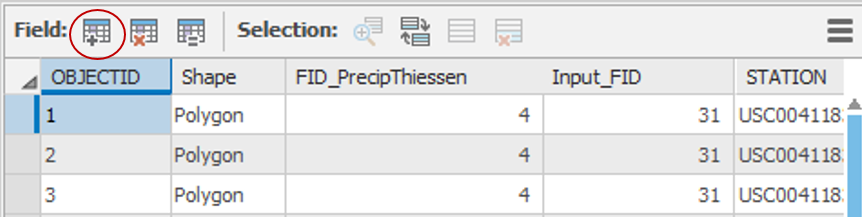
   You will add a new field to the table to calculate the elements of the numerator of the equation.|
   
   
8. Click Add Field… button on top of the table display.
   
   
   
   
9. For ‘Name:’, type “APProd”.
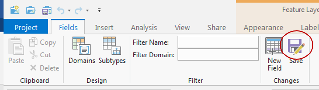
10. Use the ‘Type:’, drop-down menu to select Double and click Save on the Fields tab.
    
    
11. Right-click the APProd field name and select Calculate Field.
12. Using the fields and buttons or by typing, enter “!ANNPRCPHI! * !Shape_Area!”.

13. Ensure your ‘Field Calculator’ appears as shown below and click Run.

    
    The APProd field now contains the numerator values in the equation. You are now ready to summarize the calculated statistics by watershed.

14. Right-click the HU_10_NAME field name and select Summarize….

15. For statistics fields, use the drop-down menu to select the Shape_Area field and select Sum.

16. Select the APProd field and select Sum.
17. For ‘Output Table’, rename the table from “ThiessenWatershedInteract_St” to “WatershedPrecip”.
18. Ensure your ‘Summarize’ window appears as shown below and click Run.
    
    
    The resulting table gives the numerator and denominator in the equation for each watershed.
    
    
19. Open the WatershedPrecip table.

Repeating the techniques you just learned, add a new field to the WatershedPrecip table called “Precip” of type double. Use the field calculator to evaluate [Sum_APProd]/[Sum_Shape_Area]. The result is the precipitation for each subwatershed. Export the table to Excel and format it. Also include the mean annual precipitation over the entire watershed.

FOR TABLE TO BE TURNED IN

Create a table containing the weighted mean annual precipitation for each watershed, as calculated using Thiessen polygons, along with the total mean annual precipitation over the entire subbasin.

...

1. Turn off the ThiessenWatershedIntersect layer.
2. Right-click the Watersheds_StatePlane layer and select Zoom to Layer.
3. Open Toolbox.
4. In the Spatial Analyst Tools toolbox, click the Interpolation toolset à then the Spline tool.
5. On the top of the window, click the Environments.
6. For Extent, use the drop-down menu to select Current Display Extent.
7. Use the ‘Mask’ drop-down menu to select the Watersheds_StatePlane layer.
8. Go back to Parameters. For ‘Input point features’, drag in the PrecipStations_StatePlane layer.
9. Use the ‘Z value field’ drop-down menu to select the ANNPRCPHI field that contains the values you wish to interpolate.
10. For ‘Output raster’, rename the exported raster from “Spline_Preci1” to “AnnPrecip”.
11. Use the ‘Spline type’ drop-down menu to select TENSION.
12.  Ensure your ‘Spline’ window appears as shown below, and click Run.
    
    The result is a solid surface estimating the rainfall at each cell, based on the data collected at each rain gage. Turn the Thiessen polygons back on to give them a hollow fill. Symbolize the rain gages as you desire.

...

Using the techniques you learned earlier in this lab, use the "Zonal Statistics as Table" tool to export a table containing the total annual rainfall for each watershed, as calculated from the AnnPrecip spline interpolation layer and format the table in Excel.

FOR TABLE TO BE TURNED IN

Create a table containing the total annual precipitation for each watershed, as calculated using the spline interpolation method, along with the total annual precipitation over the entire subbasin.

...