Page History

...

1. In the Contents pane, double-click the grdn31w096_13 layer to open the 'Layer Properties' window.
2. In the Source tab, expand the 'Spatial Reference' section. scroll down and notice the spatial reference is listed as GCS_North_American_1983

Notice the Geographic Coordinate System is NAD 1983 and that no projected coordinate system is listed. Since this coordinate system is not the same as the one currently used by the data frame, the raster layer is being projected-on-the-fly into the State Plane Texas South Central projection.

Mosaicking raster files

The edges where the three tiles meet are currently visible, because the minimum and maximum elevation is different in each raster, causing the same value to be represented with a different shade of gray in each raster. To solve that visual problem and also simplify future processing steps, you will mosaic the three rasters into a single raster. Before creating a mosaic, you will need to look up a few pieces of some information from the original rasters.

1. Scroll back to the top of the ‘Layer Properties’ window and expand the 'Raster Information' section.

Notice that there is 1 band, meaning that each pixel only stores a single value: the height above sea level in meters. Aerial imagery has 3 bands to store the 3 RGB values. The format is listed as GRID, which stands for an Esri Grid, which is a raster file format native to Esri software. The pixel type and depth is 32-bit floating point, which indicates that the cells can store decimal data.

1. Close the ‘Layer Layer Properties’ window.
2. Open Tools. Click Toolboxes on the geoprocessing pane.
3. At the bottom of the Catalog pane, click the Geoprocessing tab.
4. At the top left of the Geoprocessing pane, click the Back button.
5. In the search box, type "Mosaic to New Raster".
6. Click the In the Data Management Tools toolbox, click the Raster toolset → Raster Dataset toolset → Mosaic to New Raster tool.
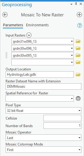
7. For ‘Input Rasters’, select the three 1x1 degree raster layers.
8. For ‘Output Location’, click the Browse button.
9. In the bottom right corner of the 'Output Location' window, use the drop-down menu to selectFile Geodatabases (instead of Folders), if necessary.
10. Select the HydrologyLab  HydrologyLab.gdb geodatabase and click AddOK.
11. For ‘Raster Dataset Name with Extension’, type “DEMMosaic”. No extension is necessary when storing the raster in a file geodatabase.
12. Use the ‘Pixel Type’ drop-down menu to select32 bit float, since that was the same type stored in the original rasters.
13. For ‘Number of Bands’, type “1”. (The text appears on the right side of the field.)
14. Ensure your ‘Mosaic To New Raster’ pane appears as shown below and click Run.
    Image Removed
    Image Added
    
    

The mosaic may take a couple minutes to process. When it is complete, notice there are no longer visual seams between the tiles in the mosaicked raster. Now that you have a single mosaic, you no longer need the three originals tiles.

1. Remove all three original raster files from the Contents paneIn the Contents pane, remove all three original raster layers.

Projecting raster files

Now you need to project your mosaic into the State Plane Texas South Central projection, so that you can properly calculate spatial statistics based on the data it contains.

1. In At the top left of the Geoprocessing pane, click Data Management Tools -> Projections and Transformations toolset -> the Raster toolset Project Raster tool. click the Back button.
2. In the search box, type "Project Raster".
3. Click the Project Raster tool.
4. Use the ‘Input Raster’ drop-down menu to select the DEMMosaic layerFor ‘Input Raster’, select in the DEMMosaic layer in the drop-down menu.
5. For ‘Output Raster Dataset’, rename the raster from “DEMMosaic_ProjectRaster” to “DEMStatePlane” DEMMosaic_ProjectRaster to “DEMStatePlane”
6. Use the For ‘Output Coordinate System’ , drop-down menu to select Watersheds_StateplaneStatePlane, which will import the same coordinate system used by that layer.

You should now see the NAD_1983_StatePlane_Texas_South_Central_FIPS_4204_Feet displayed in for the Output Coordinate System.

1. Use the ‘Resampling Technique’ drop-down menu to select Cubic Convolution.

For cell size, you may normally want to keep the original resolution, which was approximately 30 m, but, in this case, you will reduce the resolution to expedite processing times during this lab. The cell size is always specified in the same units as the projection, which in this case is feet, so you will select a cell size of 300 feet.

1. Leave ‘Output Cell Size’ blank, but­ type “300” “300” for the ‘X’ and ‘Y’. Make sure that your screen is the same as the screenshot below. Click
2. Ensure your Geoprocessing pane appears as shown and click Run.
   

Remember that the data frame was already displaying all layers in State Plane Texas South Central, so you should not notice much of a difference between the two layers, other than that the cell size has increased, meaning the resolution has decreased.

...