Page History

...

1. In the Analysis tab, click the Tools button to open the Geoprocessing pane.
2. In the 'Find Tools' search box, type "Projectproject".
3. Click the Project tool.
4. For ‘Input Dataset or Feature Class’, use the drop-down menu to select the Watersheds layer.
   
5. For ‘Output Dataset or Feature Class’, rename “Watersheds_Project” to “Watersheds_StatePlane”, since that is the name of the projection you will be using.
6. Next to the ‘Output Coordinate System’ box, click the Select Coordinate System button.
7. Double-click Projected Coordinate Systems → State Plane → NAD 1983 (US Feet).
8. Select NAD 1983 StatePlane Texas S Central FIPS 4204 (US Feet) and click OK.

...

1. Close the ‘Layer Properties’ window.
2. At the bottom of the Catalog pane, click the Geoprocessing tab.
3. At the top left of the Geoprocessing pane, click the Back button.
4. In the search box, type "Mosaic mosaic to New Rasternew raster".
5. Click the Mosaic to New Raster tool.
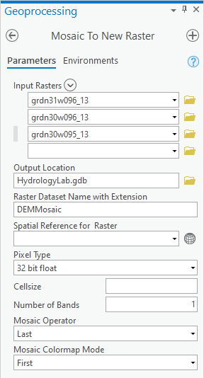
6. For ‘Input Rasters’, select the three 1x1 degree raster layers.
7. For ‘Output Location’, click the Browse button.
8. In the bottom right corner of the 'Output Location' window, use the drop-down menu to select File Geodatabases (instead of Folders), if necessary.
9. Select the HydrologyLab.gdb geodatabase and click OK.
10. For ‘Raster Dataset Name with Extension’, type “DEMMosaic”. No extension is necessary when storing the raster in a file geodatabase.
11. Use the ‘Pixel Type’ drop-down menu to select 32 bit float, since that was the same type stored in the original rasters.
12. For ‘Number of Bands’, type “1”. (The text appears on the right side of the field.)
13. Ensure your ‘Mosaic To New Raster’ pane appears as shown below and click Run.
    
    
    
    

...

1. At the top left of the Geoprocessing pane, click the Back button.
2. In the search box, type "Project Rasterproject raster".
3. Click the Project Raster tool.
4. Use the ‘Input Raster’ drop-down menu to select the DEMMosaic layer.
5. For ‘Output Raster Dataset’, rename the raster from DEMMosaic_ProjectRaster to “DEMStatePlane”
6. Use the ‘Output Coordinate System’ drop-down menu to select Watersheds_StatePlane, which will import the same coordinate system used by that layer.

...

1. At the top left of the Geoprocessing pane, click the Back button.
2. In the search box, type "Clip Rasterclip raster".
3. Click the Clip Raster tool.
4. For ‘Input Raster’, select DEMStatePlane.
5. For ‘Output Extent’, select Watersheds_StatePlane.
6. Check Use Input Features for Clipping Geometry.

...

1. At the top left of the Geoprocessing pane, click the Back button.
2. In the search box, type "Raster Calculatorraster calculator".
3. Click the Raster Calculator tool.
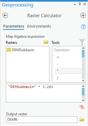
4. In the list of ‘Rasters’, double-click the DEMSubbasin layer.
5. In the list of 'Tools', double-click the * symbol.
6. In the equation box, type “3.281”, which is the conversion factor from meters to feet.
7. For ‘Output raster’, rename the raster “DEMft”.
8. Ensure your ‘Raster Calculator’ window appears as shown below and click Run.
   
   
   
   

...

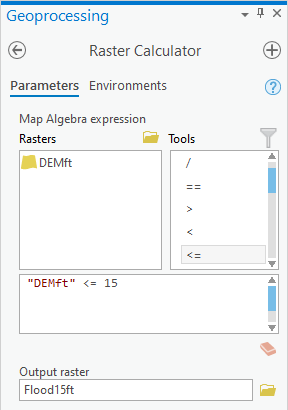
1. In the Raster Calculator tool, delete the previous expression "DEMSubbasin" * 3.281.
2. In the list of 'Rasters’, double-click the DEMft layer.
3. In the list of 'Tools', double-click the <= symbol.
4. In the equation box, type “15”.
5. For ‘Output raster’, rename the raster from demft_raster to “Flood15ft”.
6. Ensure your Geoprocessing pane appears as shown below and clickRun.
   
   
   
   
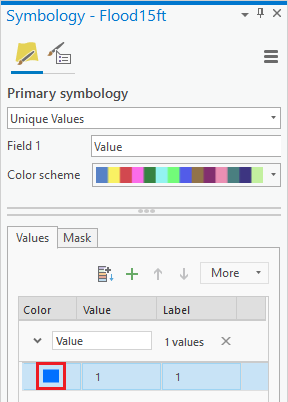
7. In the Contents pane, right-click the Flood15ft layer and select Symbology.
8. In the Symbology pane, right-click the 0 value and click Remove.
   
   
   
   
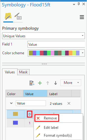
9. Click the rectangle symbol to the left of the 1 value and select Blue.
   
   
   
   

...

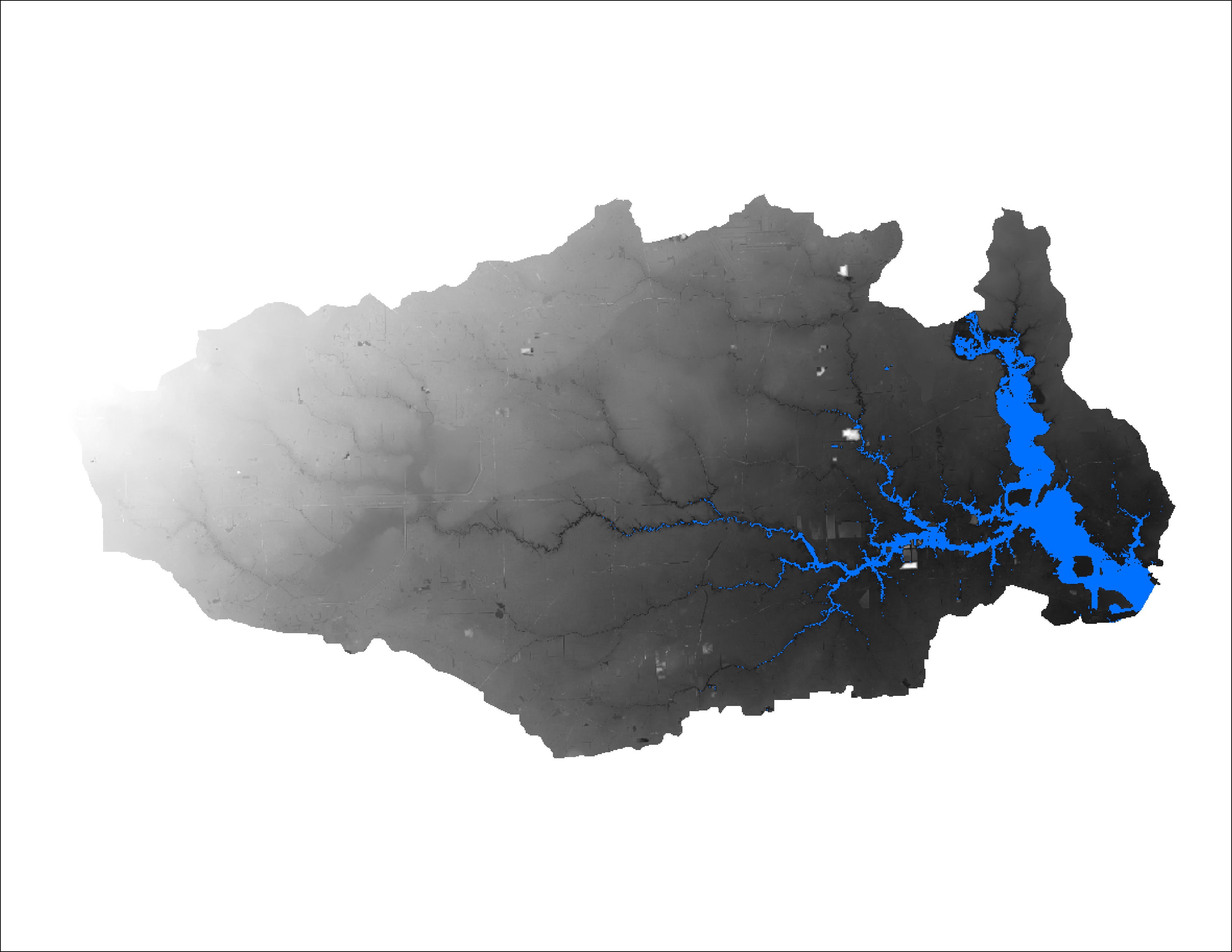
Create an 8.5 x 11 layout showing the DEM clipped to the subbasin with areas less than or equal to 15 feet in elevation highlighted.

Image RemovedImage Added

Symbolizing raster files

Now you will create a new map document from the one you are currently using.

1. On the ribbon, click the Insert tab and click the New Map button.
2. In the Contents pane, rename the map “Lab2Topo”.
3. Expand Databases in Return to the Catalog pane. Click
4. Expand the HydrologyLab.gdb geodatabase.
5. Drag the DEMft and Watersheds_StateplaneStatePlane layers into the Lab2Topo map displayview.
6. Turn off the In the Contents pane, uncheck the Watersheds_Stateplane layer.
7. Right-click the DEMft layer and click the select Symbology.
8. Scroll For ‘Color scheme’, scroll down the ‘Color Ramp’ drop-down menu to the very bottom and select the rainbow ramp Multipart Color Scheme or another continuous color scheme of your choice.
   Image Removed
   Image Added
   
   

Patterns within the data are now easier to see, especially at the lower elevations.

...

1. Return to the Geoprocessing pane.
2. At the top left of the Geoprocessing pane, click the Back button.
3. In the search box, type "Contourcontour".
4. Click the Contour (Spatial Analyst Tools) tool.
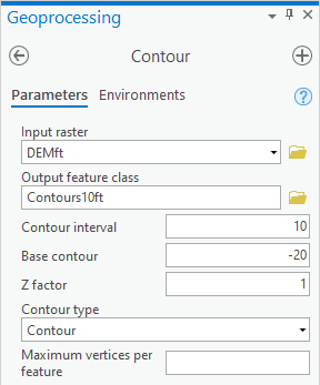
5. For ‘Input raster’, select the DEMft layer.
6. For the ‘Output polyline features’, rename the feature class from “Contour_DEMft1” to “Contours10ft”.
7. For ‘Contour interval’, type “10”.

...

1. For ‘Base contour’, type  “-20”.

Since the x,y coordinates XY coordinates are in the units of your State Plane Texas South Central projection, which is feet, and you have also used the Raster Calculator to convert the z Z units stored within the raster cells to feet, you do not need a custom Z factor.

1. For ‘Z factor’, leave the default value of 1.
2. Ensure your ‘Contour’ window Geoprocessing pane appears as shown below and clickRun.
   Image Removed
   Image Added
   
   
3. Turn off the DEMft layer to better see the contours.
4. Right-click the Contours10ft layer . Clickand select Symbology.
5. Use the In the Symbology pane, use the 'Primary symbology' drop-down menu at the top to select Unique values.
6. Use the ‘Value Field’ ‘Field 1’ drop-down menu to select the Contour field.
7. Use At the bottom of the ‘Color Ramp’ scheme’ drop-down menu. Check, check Show All and select one  one of the few graduated continuous color ramps schemes, as shown below. 
   Image Removed
   Image Added
   
   

Now you can tell which contours are highest and lowest.

1. Turn In the Contents pane, turn off and collapse the Contours10ft layer.
2. Turn back on the DEMft layer.

...

Now you will create a hillshade raster, which provides a shaded relief of the terrain based on a certain sun angle. It stores a value between 0 and 255 indicating the extent to which the cell would be shaded from the sun.

1. Return to the Geoprocessing pane.
2. At the top left of the Geoprocessing pane, click the Back button.
3. In the search box, type "hillshade".
4. Click the Hillshade (Spatial Analyst Tools) toolOpen Geoprocessing pane by clicking Tools from Analysis tab.
5. In the Surface toolset, double-click the Hillshade tool.
6. For ‘Input raster’, select the DEMft layer.
7. For ‘Output raster’, rename the raster from “HillSha_DEMf1” to “Hillshade”.

...

As previously mentioned, the Z factor is used when the horizontal units of the projection and units of the elevation measurements stored in the raster cells are not the same. In this case, both are measured in feet, so a value of 1 is technically correct. Typically, hillshades are used to create realistic three-dimensional representations of mountains, which can be much easier for an audience to interpret than a flat DEM or contour lines. Unfortunately, the opposite is true in Houston, because the area is so flat.  It would be difficult to see any changes in elevation using a hillshade, since few shadows would be cast by the terrain itself. To compensate visually for the flat terrain, you will exaggerate the vertical elevations.

1. For ‘Z factor’, type “20”.
2. Ensure your ‘Hillshade’ window appears as shown and click Run.
   Image Removed
   Image Added
   
   

Typically, hillshades are shown beneath transparent layers conveying other information, just to give the map a realistic appearance.

1. In the Contents pane, drag the Hillshade layer beneath the DEMft layer, but above the Topographic basemap.
2. In the Contents pane, select the DEMft layer.
3. In the ribbon, in click the feature-dependent contextual Appearance tab.
4. In , in the Effects group, slide the transparency to 60%.

...

1. Turn on the Watersheds_StatePlane layer.
2. Symbolize the Watersheds_StatePlane layer with no transparency, a hollow fill, and thick black outline.

As a final touch, you will add the flowlines you downloaded in Lab1 Lab 1 to your Map Display.

1. Click the Catalog tab.
2. In the HydrologyLab geodatabase, drag the Flowlines feature class into the Map Display Lap2Topo map view.
3. In the Contents pane, drag the Flowlines layer above the DEMft layer, but beneath the Watersheds_StatePlane layer.
4. Symbolize the Flowlines layer with a thin blue line.
5. Save your project.

...

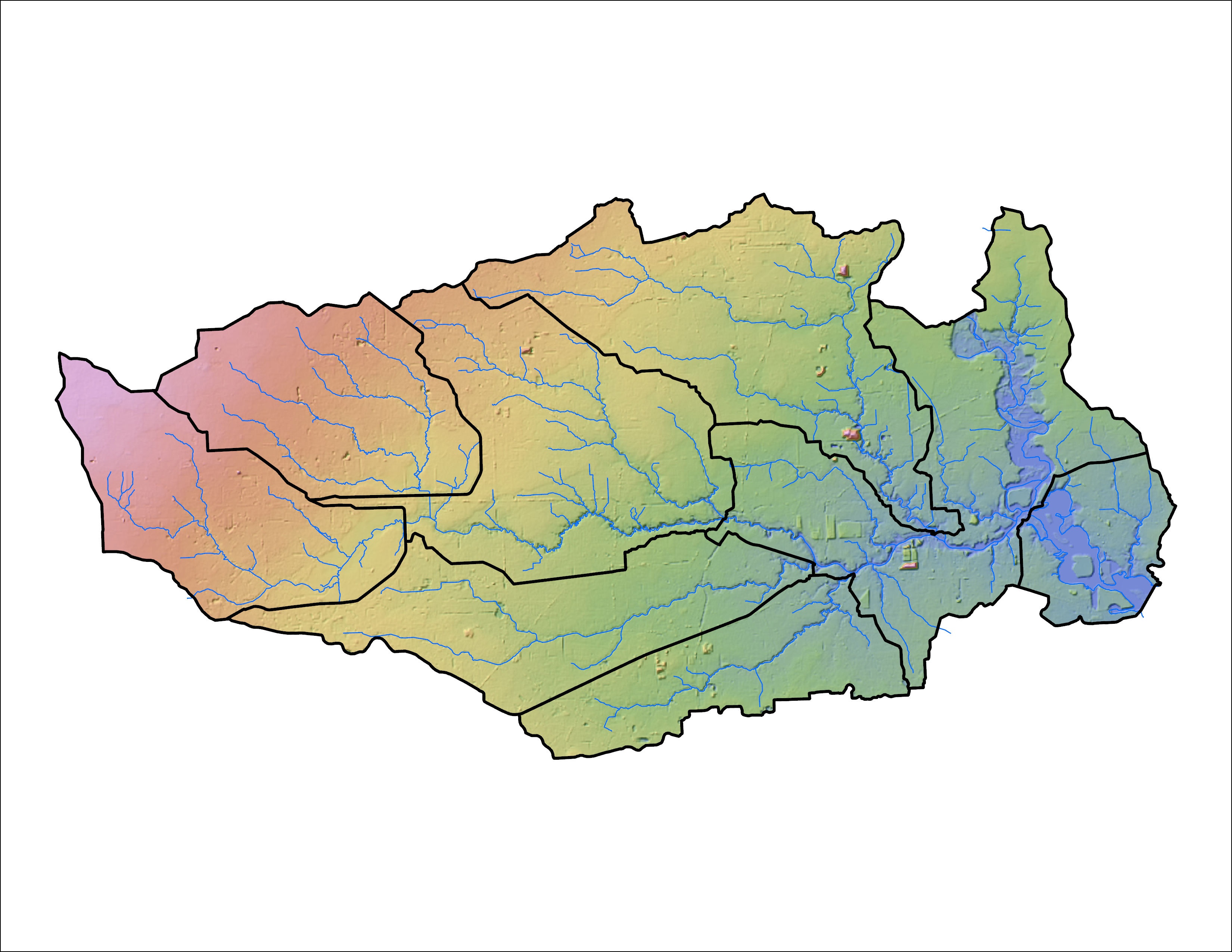
Create an 8.5 x 11 layout showing transparent elevation in graduated colors on top of a hillshade, with watershed boundaries and flowlines visible.

Image RemovedImage Added

Calculating zonal statistics

...