Page History

...

Before beginning the tutorial, you will copy all of the required tutorial data onto your Desktop. Option 1 is best if you are completing this tutorial in one of our short courses or from the GIS/Data Center and Option 2 is best if you are completing the tutorial from your own computer.

OPTION 1: Accessing tutorial data from Fondren Library using the gistrain profile

If you are completing this tutorial from a public computer in Fondren Library and are logged on using the gistrain profile, follow the instructions below:

1. On the Desktop, double-click the Computer icon > gisdata GISData (\\file-rnassmb.rdf.rice.edu\research\FondrenGDC) (RO:) >  > GDCTraining > 1_Short_Courses > > Measuring_Geographic_Distributions.
2. To create a personal copy of the tutorial data, drag the GeographicDistribution folder onto the Desktop.
3. Close all windows.

...

1. On the ribbon, click the Analysis tab.
2. On the Analysis tab, within the first Geoprocessing group, click the Tools button.
   
   Image Modified

Notice that the Geoprocessing pane has opened on the right as a new tab on top of the Catalog pane. Typically, you would use the 'Find Tools' search box at the top of the Geoprocessing pane to search for the name of the tool you'd like to use, but, at times, especially when learning the software, it can be helpful to view the full hierarchy of all the tools available, because you will often discover related and helpful tools that you didn't know existed and wouldn't know to search for. You might also completely forget the name of a tool, but be able to locate it based on the hierarchy. For these reasons, we will be manually navigating the toolboxes throughout this tutorial. The more typical workflow of searching directly for a specific tool is covered at the end of the Introduction to Geoprocessing tutorial.

...

1. In the Geoprocessing pane, click the Spatial Statistics Tools toolbox > Measuring Geographic Distributions toolset > Central Feature tool.
2. For ‘Input Feature Class’, use the drop-down menu, select the USStatesPopTimeline layer.
3. For ‘Output Feature Class’, rename the feature class "USStatesPopTimeline_CFCentralFeature_1790".
4. For ‘Weight Field,’ use the drop-down menu to select the Pop1790 field.
5. Ensure your Central Feature tool parameters are configured as shown below and click Run.
   
   

...

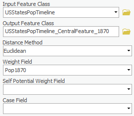
1. For ‘Output Feature Class’, rename the feature class "USStatesPopTimeline_CentralFeature_1870".
2. For ‘Weight Field,’ use the drop-down menu to select the Pop1870 field.
3. Ensure your Central Feature tool parameters are configured as shown below and click Run.
   
   

...

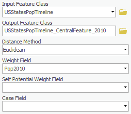
1. For ‘Output Feature Class’, rename the feature class "USStatesPopTimeline_CentralFeature_2010".
2. For ‘Weight Field,’ use the drop-down menu to select the Pop2010 field.
3. Ensure your Central Feature tool parameters are configured as shown below and click Run.
   
   

...

1. At the top of the Geoprocessing pane, click the Back arrow button.
2. Within the Measuring Geographic Distributions toolset, click the Standard Distance tool.
3. For ‘Input Feature Class’, use the drop-down menu to select the USStatesPopTimeline layer.
4. In ‘Output Standard Distance Feature Class’, rename the feature class "USStatesPopTimeline_StandardDistance_1790".
5. For ‘Circle Size’, use the drop-down menu to select 1 standard deviation.
6. For ‘Weight Field,’ use the drop-down menu to select the Pop1790 field.
7. Ensure your Standard Distance tool parameters are configured as shown below and click Run.
   
   

The result is a circle centered on Maryland. Because this circle represents one standard distance of the 1790 population, we estimate that 68% of the US population lives within that circle in 1790.

...

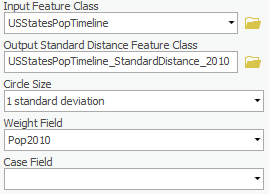
1. For ‘Output Standard Distance Feature Class’, rename the feature class "USStatesPopTimeline_StandardDistance_2010".
2. For ‘Weight Field,’ use the drop-down menu to select the Pop2010 field.
3. Ensure your Standard Distance tool parameters are configured as shown below and click Run.
   
   

...

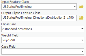
1. For ‘Output Ellipse Feature Class’, rename the feature class "USStatesPopTimeline_DirectionalDistribution2DirectionalDistribution2_1790".
2. For ‘Ellipse Size’, use the drop-down menu to select 2 standard deviations.
3. Ensure your Directional Distribution tool parameters are configured as shown below and click Run.
   
   

...

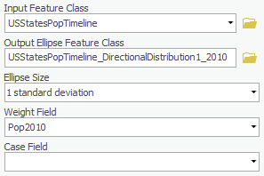
1. For ‘Output Ellipse Feature Class’, rename the feature class "USStatesPopTimeline_DirectionalDistribution1DirectionalDistribution1_2010".
2. For ‘Ellipse Size’, use the drop-down menu to select 1 standard deviation.
3. For ‘Weight Field,’ use the drop-down menu to select the Pop2010 field.
4. Ensure your Directional Distribution tool parameters are configured as shown below and click Run.
   
   

...

1. For ‘Output Ellipse Feature Class’, rename the feature class "USStatesPopTimeline_DirectionalDistribution2DirectionalDistribution2_2010".
2. For ‘Ellipse Size’, use the drop-down menu to select 2 standard deviations.
3. Ensure your Directional Distribution tool parameters are configured as shown below and click Run.
   
   

...

Road data is typically segmented , such that the length of road between each pair of intersections is a separate feature. In this tutorial, we are asking what is the average length of roadway with a single name, so the road layer was previously dissolved on the road name field, such that all road segments with the same name are were merged into a single feature. The roads layer was also clipped to approximately the extent of the Inner Loop.

...

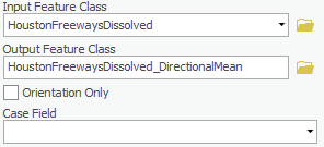
1. For the ‘Input Feature Class’, use the drop-down menu,to select the HoustonFreewaysDissolved layer.
2. For ‘Output Feature Class’, rename the feature class "HoustonFreewaysDissolved_DirectionalMean".
3. Ensure your Linear Directional Mean tool parameters are configured as shown below and click Run.
   
   
   
   
4. In the Contents pane, right-click the HoustonFreewaysDissolved layer name and select Zoom To Layer.

...