...

1. In the Analysis tab, click the Tools button to open the Geoprocessing pane.
2. In the 'Find Tools' search box, type "Projectproject".
3. Click the Project tool.
4. For ‘Input Dataset or Feature Class’, use the drop-down menu to select the Watersheds layer.
   
5. For ‘Output Dataset or Feature Class’, rename “Watersheds_Project” to “Watersheds_StatePlane”, since that is the name of the projection you will be using.
6. Next to the ‘Output Coordinate System’ box, click the Select Coordinate System button.
7. Double-click Projected Coordinate Systems → State Plane → NAD 1983 (US Feet).
8. Select NAD 1983 StatePlane Texas S Central FIPS 4204 (US Feet) and click OK.

...

1. Close the ‘Layer Properties’ window.
2. At the bottom of the Catalog pane, click the Geoprocessing tab.
3. At the top left of the Geoprocessing pane, click the Back button.
4. In the search box, type "Mosaic mosaic to New Rasternew raster".
5. Click the Mosaic to New Raster tool.
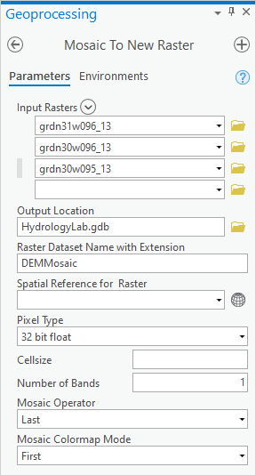
6. For ‘Input Rasters’, select the three 1x1 degree raster layers.
7. For ‘Output Location’, click the Browse button.
8. In the bottom right corner of the 'Output Location' window, use the drop-down menu to select File Geodatabases (instead of Folders), if necessary.
9. Select the HydrologyLab.gdb geodatabase and click OK.
10. For ‘Raster Dataset Name with Extension’, type “DEMMosaic”. No extension is necessary when storing the raster in a file geodatabase.
11. Use the ‘Pixel Type’ drop-down menu to select 32 bit float, since that was the same type stored in the original rasters.
12. For ‘Number of Bands’, type “1”. (The text appears on the right side of the field.)
13. Ensure your ‘Mosaic To New Raster’ pane appears as shown below and click Run.
    
    
    
    

...

1. At the top left of the Geoprocessing pane, click the Back button.
2. In the search box, type "Project Rasterproject raster".
3. Click the Project Raster tool.
4. Use the ‘Input Raster’ drop-down menu to select the DEMMosaic layer.
5. For ‘Output Raster Dataset’, rename the raster from DEMMosaic_ProjectRaster to “DEMStatePlane”
6. Use the ‘Output Coordinate System’ drop-down menu to select Watersheds_StatePlane, which will import the same coordinate system used by that layer.

...

1. At the top left of the Geoprocessing pane, click the Back button.
2. In the search box, type "Clip Rasterclip raster".
3. Click the Clip Raster tool.
4. For ‘Input Raster’, select DEMStatePlane.
5. For ‘Output Extent’, select Watersheds_StatePlane.
6. Check Use Input Features for Clipping Geometry.

...

1. At the top left of the Geoprocessing pane, click the Back button.
2. In the search box, type "Raster Calculatorraster calculator".
3. Click the Raster Calculator tool.
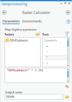
4. In the list of ‘Rasters’, double-click the DEMSubbasin layer.
5. In the list of 'Tools', double-click the * symbol.
6. In the equation box, type “3.281”, which is the conversion factor from meters to feet.
7. For ‘Output raster’, rename the raster “DEMft”.
8. Ensure your ‘Raster Calculator’ window appears as shown below and click Run.
   
   
   
   

...

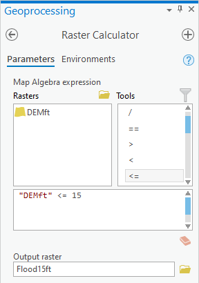
1. In the Raster Calculator tool, delete the previous expression "DEMSubbasin" * 3.281.
2. In the list of 'Rasters’, double-click the DEMft layer.
3. In the list of 'Tools', double-click the <= symbol.
4. In the equation box, type “15”.
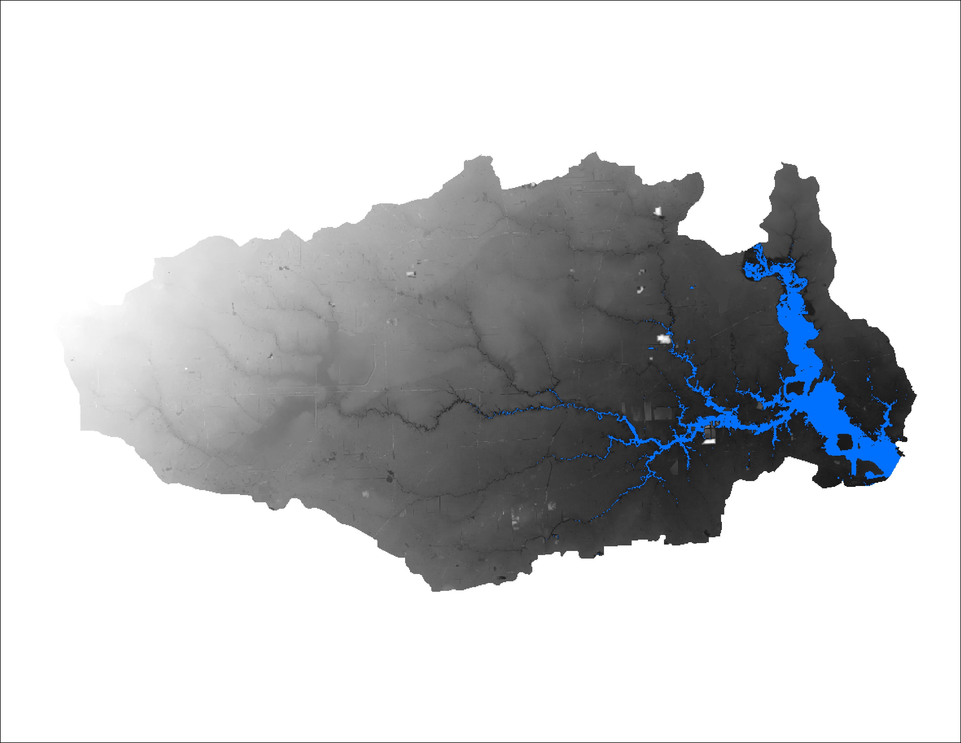
5. For ‘Output raster’, rename the raster from demft_raster to “Flood15ft”.
6. Ensure your Geoprocessing pane appears as shown below and clickRun.
   
   
   
   
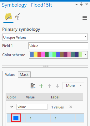
7. In the Contents pane, right-click the Flood15ft layer and select Symbology.
8. In the Symbology pane, right-click the 0 value and click Remove.
   
   
   
   
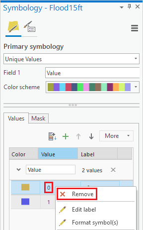
9. Click the rectangle symbol to the left of the 1 value and select Blue.
   
   
   
   

...

Create an 8.5 x 11 layout showing the DEM clipped to the subbasin with areas less than or equal to 15 feet in elevation highlighted.

Image RemovedImage Added

Symbolizing raster files

Now you will create a new map document from the one you are currently using.

1. On the ribbon, click the Insert tab and click the New Map button.
2. In the Contents pane, rename the map “Lab2Topo”.
3. Expand Databases in Return to the Catalog pane. Click
4. Expand the HydrologyLab.gdb geodatabase.
5. Drag the DEMft and Watersheds_StateplaneStatePlane layers into the Lab2Topo map displayview.
6. Turn off the In the Contents pane, uncheck the Watersheds_Stateplane layer.
7. Right-click the DEMft layer and click the select Symbology.
8. Scroll For ‘Color scheme’, scroll down the ‘Color Ramp’ drop-down menu to the very bottom and select the rainbow ramp Multipart Color Scheme or another continuous color scheme of your choice.
   Image Removed
   Image Added
   
   

Patterns within the data are now easier to see, especially at the lower elevations.

...

1. Return to the Geoprocessing pane.
2. At the top left of the Geoprocessing pane, click the Back button.
3. In the search box, type "Contourcontour".
4. Click the Contour (Spatial Analyst Tools) tool.
5. For ‘Input raster’, select the DEMft layer.
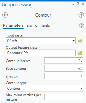
6. For the ‘Output polyline features’, rename the feature class from “Contour_DEMft1” to “Contours10ft”.
7. For ‘Contour interval’, type “10”.

...

1. For ‘Base contour’, type  “-20”.

Since the x,y coordinates XY coordinates are in the units of your State Plane Texas South Central projection, which is feet, and you have also used the Raster Calculator to convert the z Z units stored within the raster cells to feet, you do not need a custom Z factor.

1. For ‘Z factor’, leave the default value of 1.
2. Ensure your ‘Contour’ window Geoprocessing pane appears as shown below and clickRun.
   Image Removed
   Image Added
   
   
3. Turn off the DEMft layer to better see the contours.
4. Right-click the Contours10ft layer . Clickand select Symbology.
5. Use the In the Symbology pane, use the 'Primary symbology' drop-down menu at the top to select Unique values.
6. Use the ‘Value Field’ ‘Field 1’ drop-down menu to select the Contour field.
7. Use At the bottom of the ‘Color Ramp’ scheme’ drop-down menu. Check, check Show All and select one  one of the few graduated continuous color ramps schemes, as shown below. 
   Image Removed
   Image Added
   
   

Now you can tell which contours are highest and lowest.

1. Turn In the Contents pane, turn off and collapse the Contours10ft layer.
2. Turn back on the DEMft layer.

...

Now you will create a hillshade raster, which provides a shaded relief of the terrain based on a certain sun angle. It stores a value between 0 and 255 indicating the extent to which the cell would be shaded from the sun.

1. Open Return to the Geoprocessing pane by clicking Tools from Analysis tab.
2. In the Surface toolset, double-click the Hillshade tool.
3. At the top left of the Geoprocessing pane, click the Back button.
4. In the search box, type "hillshade".
5. Click the Hillshade (Spatial Analyst Tools) tool.
6. In the Surface toolset, double-click the Hillshade tool.
7. For ‘Input raster’, select the DEMft layer.
8. For ‘Output raster’, rename the raster from “HillSha_DEMf1” to “Hillshade”.

...

As previously mentioned, the Z factor is used when the horizontal units of the projection and units of the elevation measurements stored in the raster cells are not the same. In this case, both are measured in feet, so a value of 1 is technically correct. Typically, hillshades are used to create realistic three-dimensional representations of mountains, which can be much easier for an audience to interpret than a flat DEM or contour lines. Unfortunately, the opposite is true in Houston, because the area is so flat.  It would be difficult to see any changes in elevation using a hillshade, since few shadows would be cast by the terrain itself. To compensate visually for the flat terrain, you will exaggerate the vertical elevations.

1. For ‘Z factor’, type “20”.
2. Ensure your ‘Hillshade’ window appears as shown and click Run.
   Image Removed
   Image Added
   
   

Typically, hillshades are shown beneath transparent layers conveying other information, just to give the map a realistic appearance.

1. In the Contents pane, drag the Hillshade layer beneath the DEMft layer, but above the Topographic basemap.
2. In the Contents pane, select the DEMft layer.
3. In the ribbon, in click the feature-dependent contextual Appearance tab.
4. In , in the Effects group, slide the transparency to 60%.

...

1. Turn on the Watersheds_StatePlane layer.
2. Symbolize the Watersheds_StatePlane layer with no transparency, a hollow fill, and thick black outline.

As a final touch, you will add the flowlines you downloaded in Lab1 Lab 1 to your Map Display.

1. Click the Catalog tab.
2. In the HydrologyLab geodatabase, drag the Flowlines feature class into the Map Display Lap2Topo map view.
3. In the Contents pane, drag the Flowlines layer above the DEMft layer, but beneath the Watersheds_StatePlane layer.
4. Symbolize the Flowlines layer with a thin blue line.
5. Save your project.

...

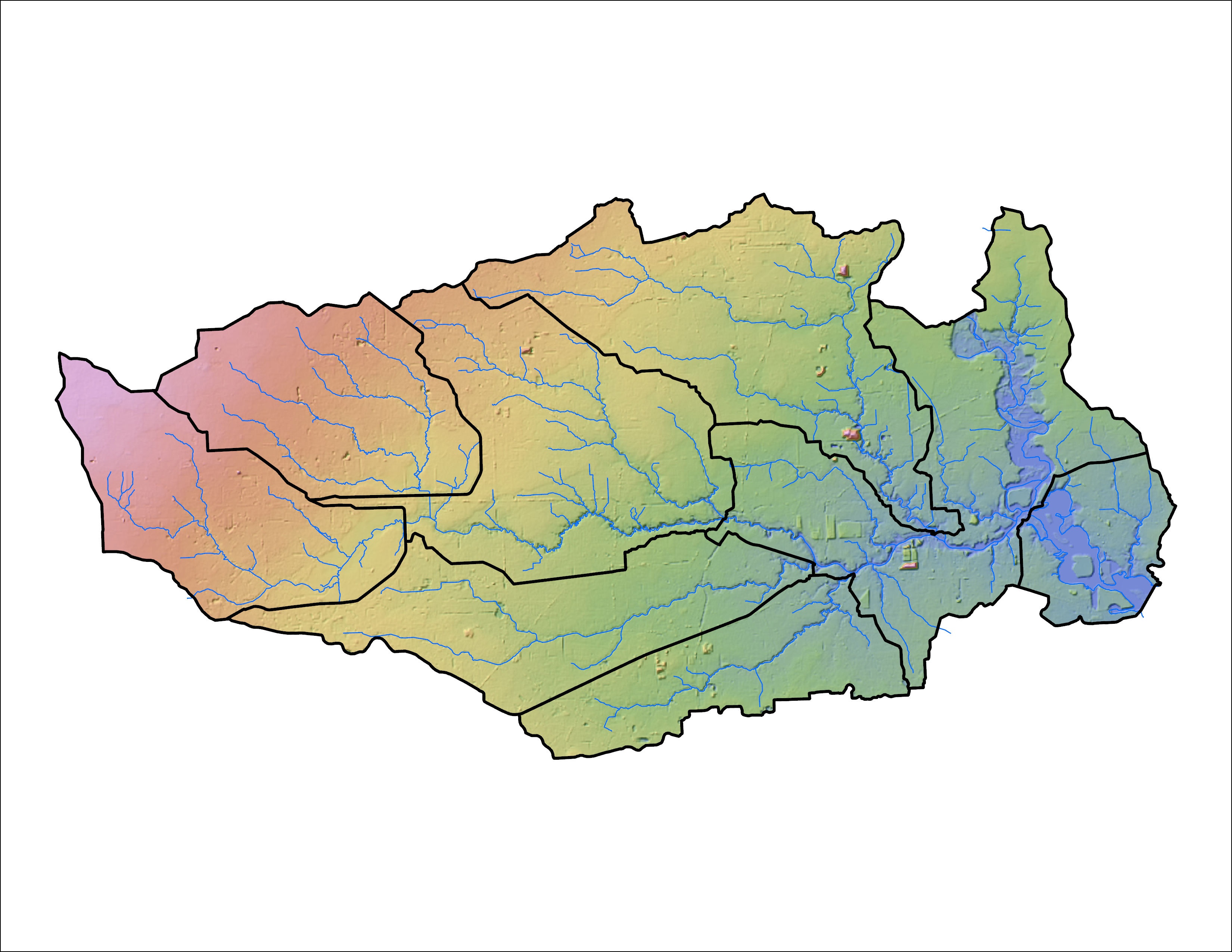
Create an 8.5 x 11 layout showing transparent elevation in graduated colors on top of a hillshade, with watershed boundaries and flowlines visible.

Image RemovedImage Added

Calculating zonal statistics

Now you will calculate elevation statistics by watershed.

1. Return to the Geoprocessing pane.
2. At the top left of the Geoprocessing pane, click the Back buttonOpen Geoprocessing pane by clicking Tools from Analysis tab.
3. In the Spatial Analyst Tools toolbox, double-click the Zonal toolset then click Zonal Statistics as Table tool.search box, type "zonal statistics".
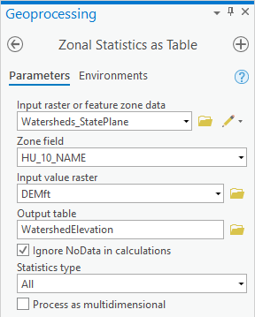
4. Click the Zonal Statistics as Table (Spatial Analyst Tools) tool.
5. Use the For ‘Input raster or feature zone data’ , use the drop-down menu to select the Watersheds_StatePlane layer.
6. Use the For ‘Zone field’ drop-down menu to , select the ‘HU_10_NAME’ field.
7. For ‘Input value raster, select the DEMft layer.
8. For ‘Output table’, rename the table from “ZonalSt_Watersh1” to “WatershedElevation”.
9. Ensure your ‘Zonal Statistics as Table’ window Geoprocessing pane appears as shown and click Run.
   Image Removed
   
   Image Added
   
   
10. At the bottom of In the Contents pane, right-click the WatershedElevation table and select Open.

This table tells you the statistics regarding all the elevation values within each watershed zone.

1. In the Geoprocessing pane, search for ‘Table "table to Excel’excel’.
2. Click the Table To Excel tool.
3. For 'For the Input Table', select WatershedElevation from the drop-down menu.
4. For ‘Output Excel File’, click the Browse button.

If you save this table inside your file geodatabase, you will not be able to open it outside of ArcGIS, so you will instead save it as a text file outside of your file geodatabase.

1. Save the table within the HydrologyLab Locate and double-click the HydrologyLab folder to save the file within the folder.
2. For ‘Name’, name as “ type “WatershedElevation”.
3. Click Save.
   
4. In the ‘Table to Excel’ windowGeoprocessing pane, click Run.
5. Close the Table WatershedElevation table.

Now you will open the exported text file in Excel.

1. Open Using File Explorer, open your WatershedElevation.xls spreadsheet in Microsoft Excel.
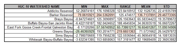
2. Delete the OBJECTID, ZONE_CODE, COUNT, AREA, and SUM fields.
3. Highlight the minimum and maximum values in each column.

...

Create a table highlighting the minimum and maximum values for the minimum, maximum, range, mean, and standard deviation of all elevation values within each watershed.

Image RemovedImage Added

Part 3: Downloading rainfall data

...

Now you will download rain gauge station data created by the National Climatic Data Center (NCDC) using the Climate Data Online (CDO) interface.

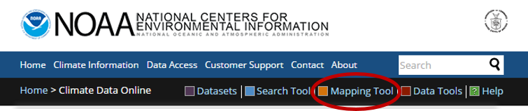
1. In a web browser, go to www.ncdc.noaa.gov/cdo-web/.
2. Click the Mapping Tool tab.
   
   
   
   

...

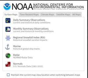
1. On the Surface Maps tab, click Normals.
   
   
   
   
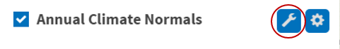
2. In the left sidebar, on the Layers tab, uncheck Daily Climate Normals, and check Annual Climate Normals.
3. To the right of Annual Climate Normals, click the Map Tools button.
   
   Image Modified
   
   
4. In the new ‘ANNUAL CLIMATE NORMALS TOOLS’ window, click Location Location.
5. Use the drop-down menu to select USGS  USGS HUC.
6. Use the ‘Select a HUC type’ drop-down menu to select Subregions  Subregions (4-digit).
7. Use the ‘Select a HUC’ drop-down menu to select Galveston  Galveston Bay-San Jacinto.
   Image Removed
   Image Added
   
   
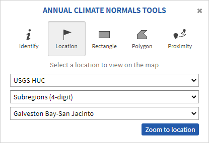
8. Click Zoom to location.
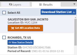
9. The left sidebar switches to the Results tab. Click Get All Location Data.
   
   
   
   
10. For Step 1, select Custom Annual/Seasonal Normals CSV for the output format and click CONTINUE.
    
    
    
    
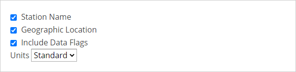
11. For ‘Station Detail & Data Flag Options’, check Station name Station Name, Geographic locationLocation, and Include data flags Data Flags to include those variables the data table.
    Image Removed
    Image Added
    
    
12. For ‘Select data types for custom output’, clickexpand the Annual Precipitation category to expand it.
13. Check Long Long-term averages of annual precipitation totals (ANN-PRCP-NORMAL).
    
    
    
    
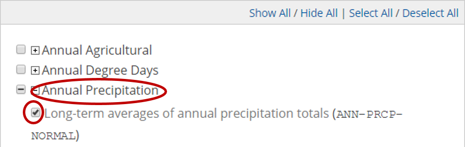
14. At the bottom of the window, click CONTINUE CONTINUE.
15. Type your email address twice and click SUBMIT  SUBMIT ORDER.

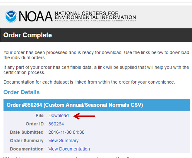
Check your email. You should receive two emails a couple minutes apart, although it may take a few hours to receive the second email. The first one indicates that your data request was submitted and the second one includes the requested data.

1. In your email, click the Download link to download the requested CSV file.
   
   

Excel

1. Navigate to the location where the CSV file was stored.
2. Double-click the CSV file to open it using Excel.

The first column contains the unique station identification code and the second column contains the station name. Next are the elevationlatitude, latitudelongitude, and longitude elevation of the stations. The annual precipitation field contains long-term averages of annual precipitation totals in hundredths of inches. More information is available on the Data Set Documentation and Samples Datasets portion of the CDO website. The annual precipitation field "

...

Before opening this table in ArcGIS, you must reformat some of the field names, which cannot have special characters and must are recommended to be 13 characters or less.

1. Rename “ANN-PRCP-NORMAL” to “ANNPRCPHIANNPRCP_HI”, for annual precipitation in hundredths of inches.
2. Along the top of the worksheet, drag across the column letters to select columns A through H F.
3. Copy the selected columns.
4. At Along the bottom left of the worksheet, click click the "plus" icon to New sheet button  to create a new sheetworksheet. In the cell A1 cell, paste your previously copied columns. 
5. Delete the previous sheet. 
6. Along the top of the worksheet, drag across the  drag across the column letters to select columns A through H F.
7. Hover your mouse between columns G E and H F until the cursor changes to two outward facing arrows and double-click to auto-size the column widths.
8. At the bottom left of the worksheet, rename the worksheet “PrecipStations”from Sheet1 to “PrecipStations”.
9. Click the File menu and select Save As.
10. Navigate to your HydrologyLab folder.
11. For ‘File name:’, type "PrecipStations".
12. Use the ‘Save as type:’ drop-down menu to select Excel 97-2003 Workbook.
13. Click Save.
14. Close Excel.

...

Now you are ready to start a new map document and display the tabular rain gage data you just downloaded.

1. Return to ArcGIS Pro.
2. Click On the Insert menu and select ribbon, click the Insert tab and click the New Map button.
3. Click “Map1” in In the contents Contents pane to rename it as “Lab2Precip”. Click Save, rename the map “Lab2Precip”.
4. Return to the Catalog pane.
5. Drag Watersheds_Stateplane onto StatePlane into the Lab2Precip map displayview.
6. Click the Geoprocessing tab and search for ‘Excel to Table’.
7. For the Input Excel File, selectPrecipStations. Rename the output table PrecipStations.
8. Right-click the HydrologyLab folder and select Refresh.
9. Expand the PrecipStations.xlsx Excel file to see the individual worksheets it contains.
10. Drag the PrecipStations$ worksheet into the Lab2Precip map viewClick Run.
11. In the Contents pane, right-click the PrecipStations PrecipStations$ table and select Display XY Data.
12. For ‘X Field:’, select the LONGITUDE field.
13. For ‘Y Field:’, select the LATITUDE field.
14. Click the Atlas to the right of the Spatial Reference boxFor 'Coordinate System', click the Select coordinate system button.

Because the coordinates are in the form of latitude and longitude in decimal degrees, you know you will need to select a geographic coordinate system, rather than a projected coordinate system.  While the data could theoretically be in any geographic coordinate system, you will select the North American Datum 1983, commonly abbreviated NAD 83, because this is coordinate system of the data provided on the NCDC website.

1. Scroll towards the top of the 'XY Coordinate Systems Available'.
2. Ensure that Geographic Coordinate Systems is already expanded, then expand Double-click Geographic Coordinate Systems > North America > USA and Territories.
3. Select NAD  NAD 1983 and click OK OK.
4. Ensure that your window matches that below and click Run OK.
   Image Removed
   Image Added

The points should now appear on top of the watersheds, though they also extend beyond the watersheds in the Buffalo-San Jacinto subbasin, since we downloaded them for the entire Galveston Bay-San Jacinto subregion.

Exporting XY data

Since the points appear to be in reasonable locations (rather than in another country or the middle of the ocean), you will want to export them to a new feature class in your ElevationRainfall geodatabase.  Exporting to a feature class will allow you to reuse this points layer in other future map documents without having to go through the display XY data process each time.

1. Right-click the PrecipStations_Layer layer and select Data > Export Features.

Because you last exported a text file outside of your geodatabase, notice the output feature class is now set to a shapefile in your Lab 2 folder, rather than a feature class within your ElevationRainfall geodatabase.

...

.

1. In the Contents pane, right-click the PrecipStations$ table and select Remove.

Projecting vector data

Repeating the technique you learned earlier in this lab to project vector data, project the PrecipStations_XYTableToPoint layer into the State Plane Texas South Central projection.Save the resulting feature class and name it

Since you are now using a permanent feature class, you may remove your temporary Events layer and the corresponding Excel table.

1. Right-click the PrecipStations_Layer layer and selectRemove.
2. Right-click the PrecipStations table and selectRemove.

Projecting vector data

Repeating the technique you learned earlier in this lab to project vector data, project the PrecipStations layer into the State Plane Texas South Central projection.Save the resulting feature class and name it “PrecipStations_StatePlane”. Remove the original PrecipStations_XYTableToPoint layer from the Contents pane.

...

1. In the Contents pane, Ctrl-select the PrecipStations_StatePlane and Watersheds_StatePlane layers.
2. Right-click either selected layer and selectZoom To Layers.
3. Open Geoprocessing pane by clicking Tools from Analysis tab.
4. Return to the Geoprocessing pane.
5. At the top left of the Geoprocessing pane, click the Back button.
6. In the search box, type "thiessen".
7. Click the Create Thiessen Polygons toolDouble-click the Analysis toolbox  then the Proximity toolset then the Create Thiessen Polygons tool.

Before populating the variables in this tool, you will change an Environment setting so that the Thiessen polygons are calculated for the entire region that you just zoomed toyou just zoomed to.

1. At the top of the Geoprocessing window, click the Environments tab on the right.
2. Under the 'Processing Extent' section, for 'Extent', select Current Display Extent.
3. At the top of the Geoprocessing window,  click the Environments tab on the right.For Extent, use the drop-down menu to select Current Display Extent and go back to Parameters return to the Parameters tab on the left.
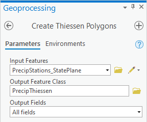
4. For ‘Input Features’,  drag in the  select the PrecipStations_StatePlane layer.
5. For ‘Output Feature Class’, rename the feature class from “PrecipStations_StatePlane_Cr” to “PrecipThiessen”.
6. Use the For ‘Output Fields’ drop-down menu to select, select All fields.
7. Ensure your ‘Create Thiessen Polygons’ window appears as shown below and click Run.
   
   Image AddedImage Removed
   
   

You will notice that polygons now fill the entire Map Display indicating which areas are closest to which rain gages.

1. Open the PrecipThiessen layer attribute table.

Notice that all of the fields that you originally downloaded from CDO are still included, because you selected to output all fields when running the Create Thiessen Polygons tool. If you do not see all of the same fields, re-run the tool and this time output all fields.

1. Close the Table PrecipThiessen attribute table.

Intersecting two polygon layers

In order to determine which portions of the resulting polygons overlap with which watersheds, you will now perform an intersect operation between the two layers. The result will allow you to calculate weighted averages of the precipitation in each watershed.

1. At the top left of the Geoprocessing pane, click the Back button.
2. In the search box, type "intersect".
3. Click the Intersect toolIn the Analysis Tools toolbox, click the Overlay toolset then the Intersect tool.
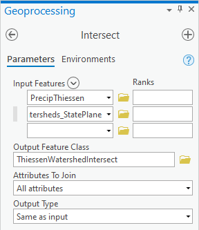
4. For ‘Input Features’, drag in the select the PrecipThiessen and the Watersheds_StatePlane layers.
5. For ‘Output Feature Class’, rename it from “PrecipThiessenPrecipThiessen_Intersect” Intersect to “ThiessenWatershedIntersect”“ThiessenWatershedIntersect”.
6. Ensure your ‘Intersect’ window appears as shown below and click Run.
   Image Removed
   Image Added
   
   
7. Remove In the Contents pane, remove the PrecipThiessen layer from the Contents pane.
8. Zoom to the ThiessenWatershedIntersect layer.

The resulting layer integrates all of the boundaries from both the Thiessen polygons and the watersheds, limited to the extent of their overlap.

1. Open the ThiessenWatershedIntersect layer attribute table.
   
   Notice that the original 8 watersheds have now been divided into 42 41 sections indicating which areas of each watershed are closest to each rain gage. Let P_k denote the annual precipitation associated with each rain gage and A_ik denote the area of the intersected polygon associated with rain gage _k and watershed _i. The area weighted precipitation associated with each watershed is
   Image Removed
   Image Added
   You will add a new field to the table to calculate the elements of the numerator of the equation.|
   
   
   
2. At the top left of the attribute table, click the Click Add Field… button on top , which will open up the Fields view of the table display.
   
   
   
   
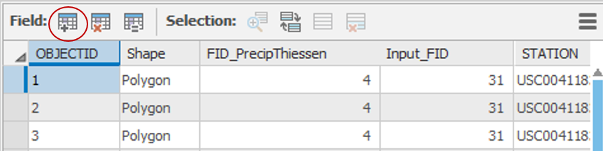
3. For ‘Name:’, type “APProd”At the bottom of the Fields table, rename the new field from Field to “APProd”.
4. Use the ‘Type:’, ‘Data Type’ drop-down menu to select Double and click.
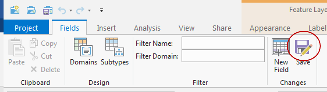
5. On the Ribbon, Save on the Fields tab, click the Save button.
   
   
   
   
6. Close the Fields view of the table.
7. Scroll to the far right of the ThiessenWatershedIntersect table.
8. Right-click the APProd field name and select Calculate  Calculate Field.
9. Using the fields and buttons or by typing, enter “!ANNPRCPHI! * !Shape_Area!”.
10. In the 'Fields' list, double-click ANNPRCP_HI.
11. Underneath the 'Helpers' list, click the * button.
12. In the 'Fields' list, double-click Shape_Area.

13. Ensure your ‘Calculate Field’ window Ensure your ‘Field Calculator’ appears as shown below and click Run OK.

    Image Removed

    Image Added

The APProd field now contains the numerator values in the equation. You are now ready to summarize the calculated statistics by watershed.

...

1. Right-click the HU_10_NAME field name and select Summarize… Summarize.

2. For ‘Output Table’, rename the table from ThiessenWatershedInteract_S to “WatershedPrecip”.

3. For statistics fields'Statistics Field(s)', use the drop-down menu to select the Shape_Area field and select Sum.

4. Select the APProd field and select Sum.
5. For ‘Output Table’, rename the table from “ThiessenWatershedInteract_St” to “WatershedPrecip”.

6.  'Field' and the Sum 'Statistic Type'.

7. For the second statistics field, select the APProd 'Field' and the Sum 'Statistic Type'.
8. Ensure the 'Case field' is the HU_10_NAME field, which will summarize the statistics by watershed.
9. Ensure your 'Summary Statistics" Ensure your ‘Summarize’ window appears as shown below and click Run OK.
   Image Removed
   Image Added
   
   

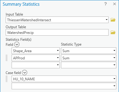
The resulting table gives the numerator and denominator in the equation for each watershed.

1. Open the WatershedPrecip table.

Repeating the techniques you just learned, add a new field to the WatershedPrecip table called “Precip” of type double. Use the field calculator to evaluate [Sum_APProd]/[Sum_Shape_Area]. The result is the precipitation for each subwatershed. Export the table to Excel and format it. Also include the mean annual precipitation over the entire watershed.

...

Now you will calculate precipitation for each watershed using a different interpolation method.

1. Close the WatershedPrecip table and the ThiessenWatershedIntersect attribute table.
2. Turn off the ThiessenWatershedIntersect layer.
3. Right-click the Watersheds_StatePlane layer and select Zoom to Layer.
4. Open ToolboxAt the top left of the Geoprocessing pane, click the Back button.
5. In the search box, type "spline".
6. Click the Spline (Spatial Analyst Tools toolbox, click the Interpolation toolset then the Spline ) tool.
7. On At the top of the Geoprocessing window, click the Environments tab. the Environments tab on the right.
8. Under the 'Processing Extent' section, for 'Extent', select For Extent, use the drop-down menu to select Current Display Extent.
9. Use the ‘Mask’ drop-down menu to select the Watersheds_StatePlane layer.
10. Under the 'Raster Analysis' section, for ‘Mask', select the Watersheds_StatePlane layer, which will clip the resulting raster.
11. At the top of the Geoprocessing window, return to the Parameters tab on the left.
12. Go back to Parameters. For ‘Input point features’, drag in the select the PrecipStations_StatePlane layer.
13. Use the For ‘Z value field’ drop-down menu to , select the ANNPRCPHI ANNPRCP_HI field that contains the values you wish to interpolate.
14. For ‘Output raster’, rename the exported raster from “SplineSpline_Preci1” to Preci1 to “AnnPrecip”.
15. Use the For ‘Spline type’ drop-down menu to select TENSION, select Tension.
16.  Ensure your Geoprocessing pane appears as shown below, and click Run.
    Image Removed
    Image Added
    
    

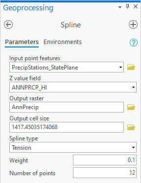
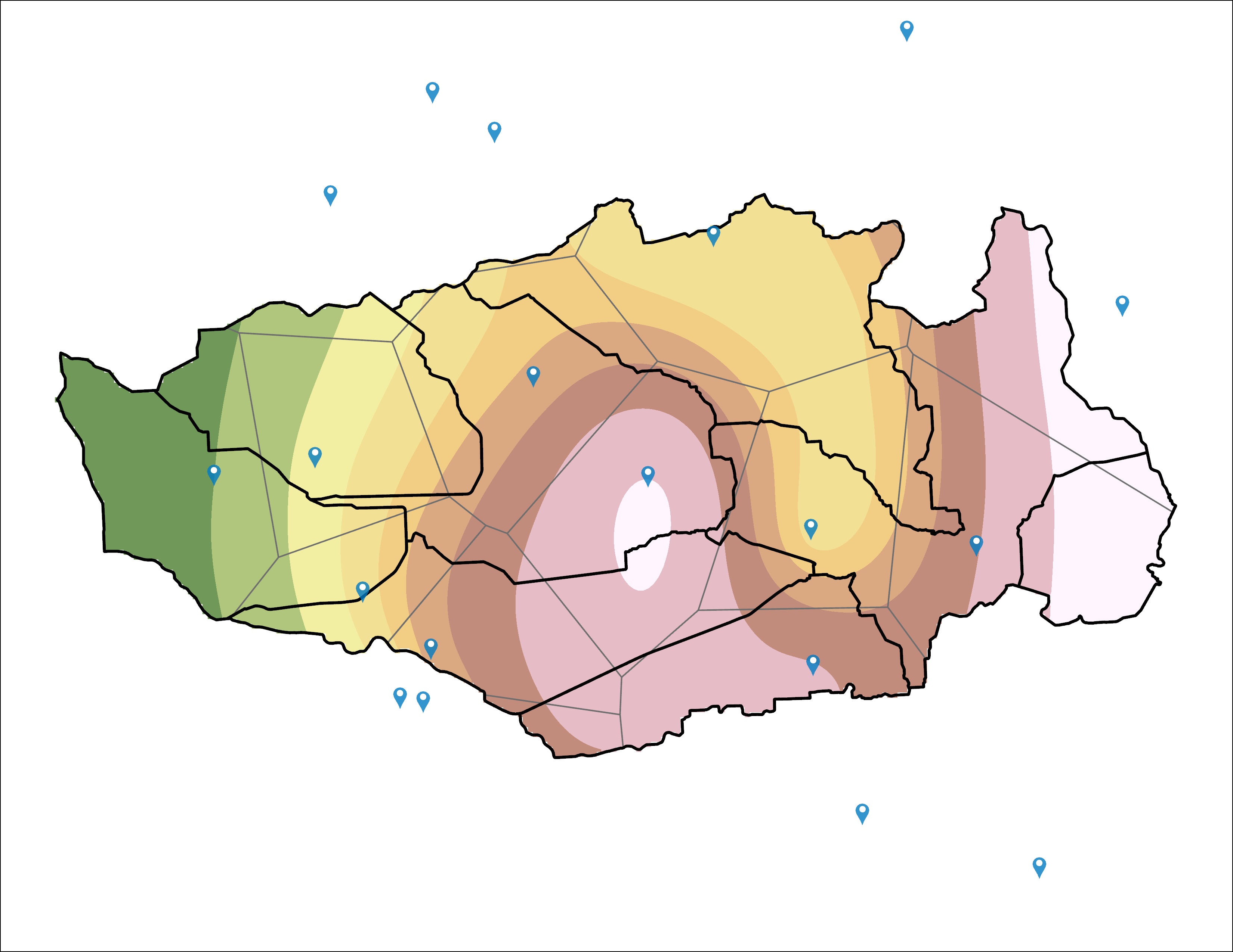
The result is a solid surface estimating the rainfall at each cell, based on the data collected at each rain gage. Turn the Thiessen ThiessenWatershedIntersect polygons back on to and give them a hollow fill. Also symbolize the Watersheds_StatePlane layer and put it on top of the Thiessen layer. Symbolize the rain gages as you desire.

...

Create an 8.5 x 11 layout showing the Thiessen polygon boundaries, interpolated rainfall layer and rain gage locations.

TOP MAP WAS THE ORIGINAL MAP, BOTTOM IS MY SCREENSHOT WHICH HAS SOMEWHAT DIFFERENT DATA. NOT SURE IF IT MATTERS BUT THOUGHT IT WORTHWHILE TO AT LEAST CHECK

Image Removed

Image Removed

Image Added

Using the techniques you learned earlier in this lab, use the " Zonal Statistics as Table " tool to export a table containing the total annual rainfall for each watershed, as calculated from the AnnPrecip spline interpolation layer and format the table in Excel.

...