Page History

...

1. In the Analysis tab, click the Tools button to open the Geoprocessing pane.
2. In the 'Find Tools' search box, type "project".
3. Click the Project tool.
4. For ‘Input Dataset or Feature Class’, use the drop-down menu to select the Watersheds layer.
   
5. For ‘Output Dataset or Feature Class’, rename “Watersheds_Project” to “Watersheds_StatePlane”, since that is the name of the projection you will be using.
6. Next to the ‘Output Coordinate System’ box, click the Select Coordinate System button.
7. Double-click Projected Coordinate Systems → State Plane → NAD 1983 (US Feet).
8. Select NAD 1983 StatePlane Texas S Central FIPS 4204 (US Feet) and click OK.

...

1. On the ribbon, click the Insert tab and click the New Map button.
2. In the Contents pane, rename the map “Lab2Topo”.
3. Return to the Catalog pane.
4. Expand the HydrologyLab.gdb geodatabase.
5. Drag the DEMft and Watersheds_StatePlane layers into the Lab2Topo map view.
6. In the Contents pane, uncheck the Watersheds_Stateplane layer.
7. Right-click the DEMft layer and select Symbology.
8. For ‘Color scheme’, scroll down to the very bottom and select the Multipart Color Scheme or another continuous color scheme of your choice.
   
   
   
   

...

Now you are ready to start a new map and display the tabular rain gage data you just downloaded.

1. Return to ArcGIS Pro.
2. Click On the Insert menu and select ribbon, click the Insert tab and click the New Map button.
3. Click “Map1” in In the contents Contents pane to rename it as , rename the map “Lab2Precip”. Click Save
4. Return to the Catalog pane.
5. Drag Watersheds_StatePlane onto  into the Lab2Precip map displayview.
6. Click the Geoprocessing tab and search for ‘Excel to Table’.
7. For the Input Excel File, selectPrecipStations. Rename the output table PrecipStations.
8. Right-click the HydrologyLab folder and select Refresh.
9. Expand the PrecipStations.xlsx Excel file to see the individual worksheets it contains.
10. Drag the PrecipStations$ worksheet into the Lab2Precip map viewClick Run.
11. In the Contents pane, right-click the PrecipStations PrecipStations$ table and select Display XY Data.
12. For ‘X Field:’, select the LONGITUDE field.
13. For ‘Y Field:’, select the LATITUDE field.
14. For 'Spatial ReferenceCoordinate System', click the Browse Select coordinate system button.

Because the coordinates are in the form of latitude and longitude in decimal degrees, you know you will need to select a geographic coordinate system, rather than a projected coordinate system.  While the data could theoretically be in any geographic coordinate system, you will select the North American Datum 1983, commonly abbreviated NAD 83, because this is coordinate system of the data provided on the NCDC website.

1. Scroll towards the top of the 'XY Coordinate Systems Available'.
2. Ensure that Double-click Geographic Coordinate Systems > is already expanded, then expand North America > USA and Territories.
3. Select NAD 1983 and click OK.
4. Ensure that your window matches that below and click RunOK.
   Image Removed
   Image Added

The points should now appear on top of the watersheds, though they also extend beyond the watersheds in the Buffalo-San Jacinto subbasin, since we downloaded them for the entire Galveston Bay-San Jacinto subregion.

Exporting XY data

Since the points appear to be in reasonable locations (rather than in another country or the middle of the ocean), you will want to export them to a new feature class in your ElevationRainfall geodatabase.  Exporting to a feature class will allow you to reuse this points layer in other future map documents without having to go through the display XY data process each time.

1. Right-click the PrecipStations_Layer layer and select Data > Export Features.

Because you last exported a text file outside of your geodatabase, notice the output feature class is now set to a shapefile in your Lab 2 folder, rather than a feature class within your ElevationRainfall geodatabase.

...

.

1. In the Contents pane, right-click the PrecipStations$ table and select Remove.

Projecting vector data

Repeating the technique you learned earlier in this lab to project vector data, project the PrecipStations_XYTableToPoint

Since you are now using a permanent feature class, you may remove your temporary Events layer and the corresponding Excel table.

1. Right-click the PrecipStations_Layer layer and select Remove.
2. Right-click the PrecipStations table and select Remove.

Projecting vector data

Repeating the technique you learned earlier in this lab to project vector data, project the PrecipStations layer into the State Plane Texas South Central projection.Save the resulting feature class and name it “PrecipStations_StatePlane”. Remove the original PrecipStations_XYTableToPoint layer from the Contents pane.

...

1. In the Contents pane, Ctrl-select the PrecipStations_StatePlane and Watersheds_StatePlane layers.
2. Right-click either selected layer and selectZoom To Layers.
3. Return to the Geoprocessing pane.
4. Open Geoprocessing pane by clicking Tools from Analysis tab.
5. At the top left of the Geoprocessing pane, click the Back button.
6. In the search box, type "thiessen".
7. Click the Create Thiessen Polygons toolDouble-click the Analysis toolbox  then the Proximity toolset then the Create Thiessen Polygons tool.

Before populating the variables in this tool, you will change an Environment setting so that the Thiessen polygons are calculated for the entire region that you just zoomed to.

1. At the top of the Geoprocessing window, click the Environments tab on the right.
2. Under the 'Processing Extent' section, for 'Extent', select Current Display Extent.
3. At the top of the Geoprocessing window, return to the Parameters tab on the leftFor Extent, use the drop-down menu to select Current Display Extent and go back to Parameters.
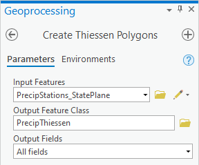
4. For ‘Input Features’,  drag in the  select the PrecipStations_StatePlane layer.
5. For ‘Output Feature Class’, rename the feature class from “PrecipStations_StatePlane_Cr” to “PrecipThiessen”.
6. Use the For ‘Output Fields’ drop-down menu to , select All fields.
7. Ensure your ‘Create Thiessen Polygons’ window appears as shown below and click Run.
   
   Image AddedImage Removed
   
   

You will notice that polygons now fill the entire Map Display indicating which areas are closest to which rain gages.

...

Notice that all of the fields that you originally downloaded from CDO are still included, because you selected to output all fields when running the Create Thiessen Polygons tool. If you do not see all of the same fields, re-run the tool and this time output all fields.

1. Close the Table PrecipThiessen attribute table.

Intersecting two polygon layers

In order to determine which portions of the resulting polygons overlap with which watersheds, you will now perform an intersect operation between the two layers. The result will allow you to calculate weighted averages of the precipitation in each watershed.

1. At the top left of the Geoprocessing pane, click the Back button.
2. In the search box, type "intersect".
3. Click the Intersect toolIn the Analysis Tools toolbox, click the Overlay toolset then the Intersect tool.
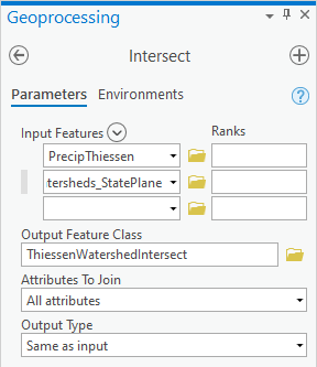
4. For ‘Input Features’, drag in the select the PrecipThiessen and the Watersheds_StatePlane layers.
5. For ‘Output Feature Class’, rename it from PrecipThiessen_Intersect to “ThiessenWatershedIntersect”.
6. Ensure your ‘Intersect’ window appears as shown below and click Run.
   Image Removed
   Image Added
   
   
7. Remove In the Contents pane, remove the PrecipThiessen layer from the Contents pane.
8. Zoom to the ThiessenWatershedIntersect layer.

...

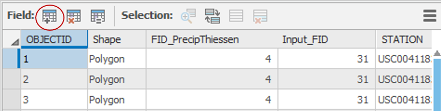
1. Open the ThiessenWatershedIntersect layer attribute table.
   
   Notice that the original 8 watersheds have now been divided into 42 41 sections indicating which areas of each watershed are closest to each rain gage. Let P_k denote the annual precipitation associated with each rain gage and A_ik denote the area of the intersected polygon associated with rain gage _k and watershed _i. The area weighted precipitation associated with each watershed is
   Image Removed
   Image Added
   You will add a new field to the table to calculate the elements of the numerator of the equation.|
   
   
   
2. At the top left of the attribute table, clickClick the Add Field… button on top , which will open up the Fields view of the table display.
   
   
   
   
3. For ‘Name:’, type At the bottom of the Fields table, rename the new field from Field to “APProd”.
4. Use the ‘Type:’, ‘Data Type’ drop-down menu to select Double and click.
5. On the Ribbon, Save on the Fields tab, click the Save button.
   
   
   
   
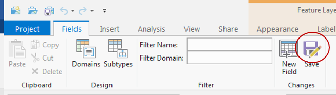
6. Close the Fields view of the table.
7. Scroll to the far right of the ThiessenWatershedIntersect table.
8. Right-click the APProd field name and select Calculate Field.
9. Using the fields and buttons or by typing, enter “!ANNPRCPHI! * !Shape_Area!”.
10. .
11. In the 'Fields' list, double-click ANNPRCP_HI.
12. Underneath the 'Helpers' list, click the * button.
13. In the 'Fields' list, double-click Shape_Area.

14. Ensure your ‘Calculate Field’ window Ensure your ‘Field Calculator’ appears as shown below and clickRun OK.Image Removed

    Image Added

The APProd field now contains the numerator values in the equation. You are now ready to summarize the calculated statistics by watershed.

1. Right-click the HU_10_NAME field name and select Summarize…Summarize.

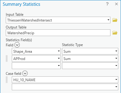
2. For ‘Output Table’, rename the table from ThiessenWatershedInteract_S to “WatershedPrecip”.

3. For statistics fields'Statistics Field(s)', use the drop-down menu to select the Shape_Area field and select Sum.

4. Select the APProd field and select Sum.
5. For ‘Output Table’, rename the table from ThiessenWatershedInteract_St to “WatershedPrecip”.

6.  'Field' and the Sum 'Statistic Type'.

7. For the second statistics field, select the APProd 'Field' and the Sum 'Statistic Type'.
8. Ensure the 'Case field' is the HU_10_NAME field, which will summarize the statistics by watershed.
9. Ensure your 'Summary Statistics" window Ensure your Geoprocessing pane appears as shown below and click RunOK.
   Image Removed
   Image Added
   
   

The resulting table gives the numerator and denominator in the equation for each watershed.

...

Now you will calculate precipitation for each watershed using a different interpolation method.

1. Close the WatershedPrecip table and the ThiessenWatershedIntersect attribute table.
2. Turn off the ThiessenWatershedIntersect layer.
3. Right-click the Watersheds_StatePlane layer and select Zoom to Layer.
4. Open Toolbox.
5. In the Spatial Analyst Tools toolbox, click the Interpolation toolset then the Spline tool.
6. At the top left of the Geoprocessing pane, click the Back button.
7. In the search box, type "spline".
8. Click the Spline (Spatial Analyst Tools) tool.
9. At On the top of the Geoprocessing window, click the Environments tab. the Environments tab on the right.
10. Under the 'Processing Extent' section, for 'Extent', select For Extent, use the drop-down menu to select Current Display Extent.
11. Use the ‘Mask’ drop-down menu to select the Watersheds_StatePlane layer.
12. Under the 'Raster Analysis' section, for ‘Mask', select the Watersheds_StatePlane layer, which will clip the resulting raster.
13. At the top of the Geoprocessing window, return to the Parameters tab on the left.
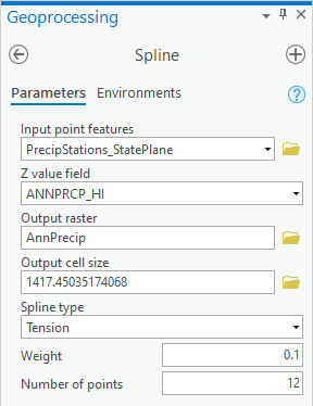
14. Go back to Parameters. For ‘Input point features’, drag in the select the PrecipStations_StatePlane layer.
15. Use the For ‘Z value field’ drop-down menu to , select the ANNPRCPHI ANNPRCP_HI field that contains the values you wish to interpolate.
16. For ‘Output raster’, rename the exported raster from Spline_Preci1 to “AnnPrecip”.
17. Use the For ‘Spline type’ drop-down menu to select TENSION, select Tension.
18.  Ensure your Geoprocessing pane appears as shown below, and click Run.
    Image Removed
    Image Added
    
    

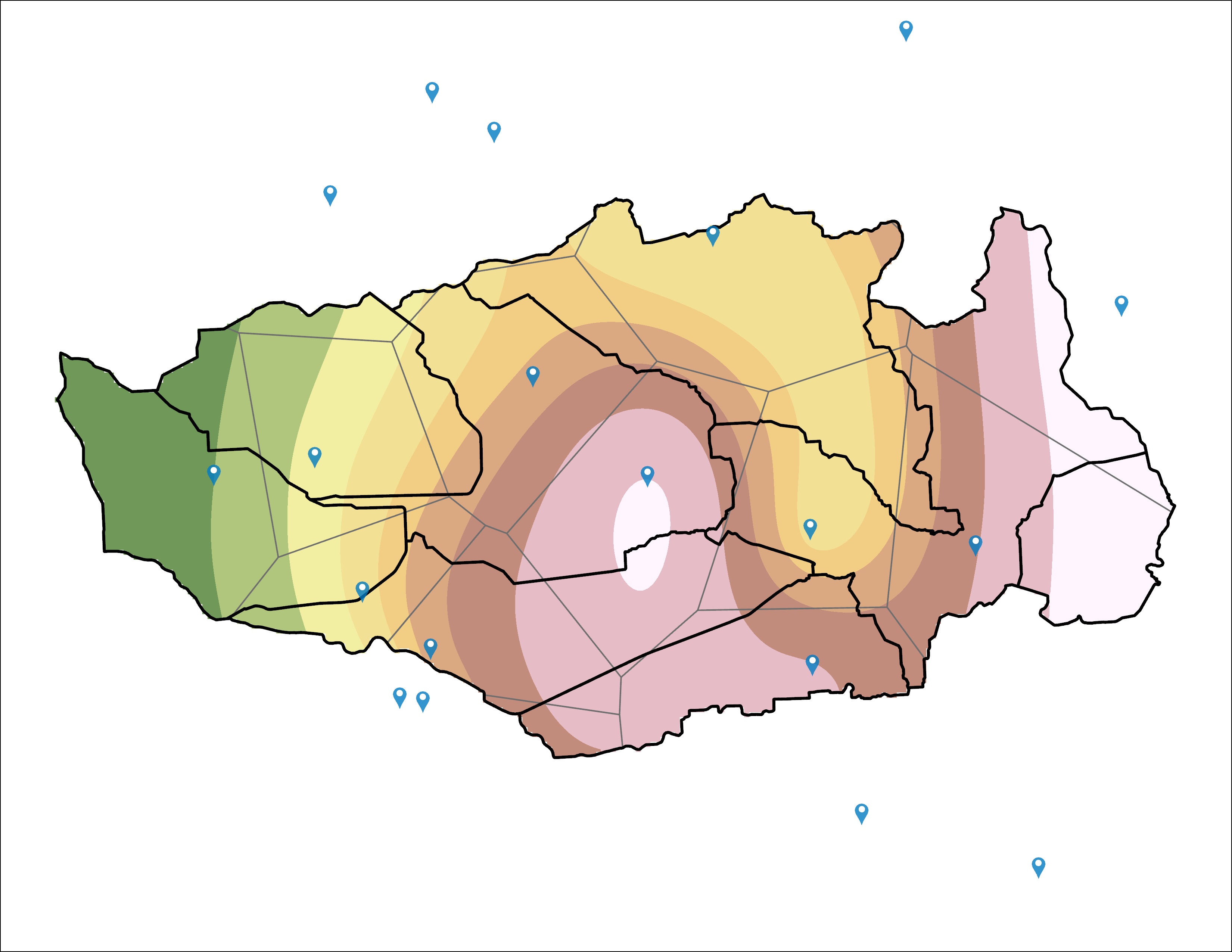
The result is a solid surface estimating the rainfall at each cell, based on the data collected at each rain gage. Turn the Thiessen ThiessenWatershedIntersect polygons back on to and give them a hollow fill. Also symbolize the Watersheds_StatePlane layer and put it on top of the Thiessen layer. Symbolize the rain gages as you desire.

...

Create an 8.5 x 11 layout showing the Thiessen polygon boundaries, interpolated rainfall layer and rain gage locations.

TOP MAP WAS THE ORIGINAL MAP, BOTTOM IS MY SCREENSHOT WHICH HAS SOMEWHAT DIFFERENT DATA. NOT SURE IF IT MATTERS BUT THOUGHT IT WORTHWHILE TO AT LEAST CHECK

Image Removed

Image Removed

Image Added

Using the techniques you learned earlier in this lab, use the " Zonal Statistics as Table " tool to export a table containing the total annual rainfall for each watershed, as calculated from the AnnPrecip spline interpolation layer and format the table in Excel.

...