...
Create an 8.5 x 11 layout showing transparent elevation in graduated colors on top of a hillshade, with watershed boundaries and flowlines visible.

Calculating zonal statistics
...
- Open Geoprocessing pane by clicking Tools from Analysis tab.
- In the Spatial Analyst Tools toolbox, double-click the Zonal toolset à Zonal Statistics as Table tool.
- For ‘Input raster or feature zone data’, use the drop-down menu to select the Watersheds_StatePlane layer.
- Use the ‘Zone field’ drop-down menu to select the ‘HU_10_NAME’ field.
- For ‘Input value raster, select the DEMft layer.
- For ‘Output table’, rename the table from “ZonalSt_Watersh1” to “WatershedElevation”.
- Ensure your ‘Zonal Statistics as Table’ window appears as shown and click Run.
...

- In the Table of Contents, right-click the WatershedElevation table and select Open.
...
Create a table highlighting the minimum and maximum values for the minimum, maximum, range, mean, and standard deviation of all elevation values within each watershed.

Part 3: Downloading rainfall data
...
- In a web browser, go to www.ncdc.noaa.gov/cdo-web/.
- Click the Mapping Tool tab.
...
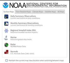
You will search for data using the NHD hydrologic units. Previously, you had been working with the Buffalo-San Jacinto subbasin (HUC = 12040104). In this case, you will step up two levels to the Galveston Bay-San Jacinto subregion (HUC = 1204).- On the Surface Maps tab, click Normals
...
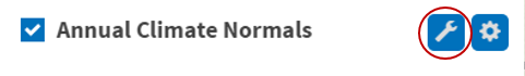
- In the left sidebar, on the Layers tab, uncheck Daily Daily Climate Normals and and check Annual Annual Climate Normals
- To the right of Annual Climate Normals, click click the Map Tools button.
...
- In the new ‘ANNUAL CLIMATE NORMALS TOOLS’ window, click Location Location.
- Use the drop-down menu to to select USGS USGS HUC.
- Use the ‘Select a HUC type’ drop-down menu to to select Subregions Subregions (4-digit).
- Use the ‘Select a HUC’ drop-down menu to to select Galveston Galveston Bay-San Jacinto.
...

...
- Click
...
- Zoom to location.
...
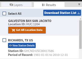
- The left sidebar switches to the Results tab. Click
...
- Get All Location Data.
...
- For Step 1, select CSV for the output format and click CONTINUE.
...

...
- For ‘Station Detail & Data Flag Options’, check
...
- Station name, Geographic location, and Include data flags to include those variables the data table.
...

...
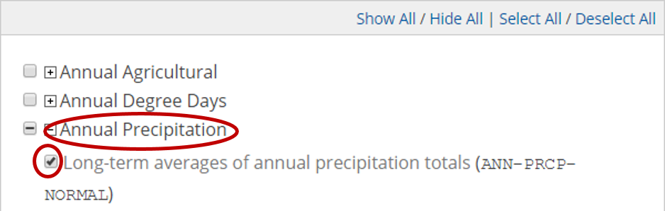
- For ‘Select data types for custom output’, click
...
- the Annual Precipitation category to expand it.
...
- Check
...
- Long-term averages of annual precipitation totals (ANN-PRCP-NORMAL).
...
- 16. At At the bottom of the window, click CONTINUE CONTINUE.
...
- Type
...
- your email address twice
...
- and click
...
- SUBMIT ORDER.
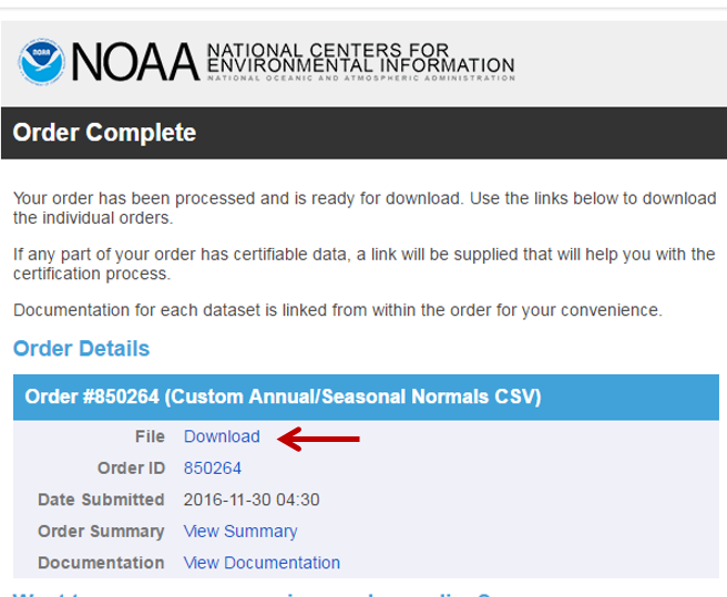
Check your email. You should receive two emails a couple minutes apart, although it may take a few hours to receive the second email. The first one indicates that your data request was submitted and the second one includes the requested data.
...
- In your email, click
...
- the Download link to download the requested CSV file.
...
Excel
- Navigate to the location where the CSV file was stored.
- Double-click the CSV file to open it using Excel.
- Along the top of the worksheet, drag across the column letters to select columns A through H.
- Hover your mouse between columns G and H until the cursor changes to two outward facing arrows and double-click to auto-size the column widths.
...
- Return to ArcGIS Pro.
- Click the Insert menu and select New Map….
- Click “Map1” in the contents pane to rename it as “Lab2Precip”. Click Save.
- Drag Watersheds_Stateplane onto the map display.
- Click the Geoprocessing tab and search for ‘Excel to Table’.
- For the Input Excel File, select PrecipStations. Rename the output table PrecipStations.
- Click Run.
- In the Table of Contents, right-click the PrecipStations table and select Display XY Data.
- For ‘X Field:’, select the LONGITUDE field.
...
- For ‘Y Field:’, select
...
- the LATITUDE
...
- field.
Notice in the ‘Coordinate System of Input Coordinates’ box, it defaults to the particular projection being displayed in our active data frame, which is currently State Plane Texas South Central. In order to use this default projection, the XY coordinates in your spreadsheet would have to be large coordinate numbers measured in feet, but since they are provided in geographic coordinates of latitudes between -90 and 90 and longitudes between -180 and 180, you will need to specify a geographic coordinate system, rather than a projected coordinate system.
...
- Click
...
- the Atlas to the right of the Spatial Reference box.
Because the coordinates are in the form of latitude and longitude in decimal degrees, you know you will need to select a geographic coordinate system, rather than a projected coordinate system. While the data could theoretically be in any geographic coordinate system, you will select the North American Datum 1983, commonly abbreviated NAD 83, because this is coordinate system of the data provided on the NCDC website.
...
- Double-click
...
- Geographic Coordinate Systems > North America > USA and Territories.
...
- Select
...
- NAD 1983
...
- and click
...
- OK.
...
- Ensure that your window matches that below
...
- and click
...
- Run.
...

The points should now appear on top of the watersheds, though they also extend beyond the watersheds in the Buffalo-San Jacinto subbasin, since we downloaded them for the entire Galveston Bay-San Jacinto subregion.
Exporting XY data
Since the points appear to be in reasonable locations (rather than in another country or the middle of the ocean), you will want to export them to a new feature class in your ElevationRainfall geodatabase. Exporting to a feature class will allow you to reuse this points layer in other future map documents without having to go through the display XY data process each time.
...