Page History

...

A map is a project item used to display and work with geographic data in two dimensions. The first step to visualizing any data is creating a new map. The ribbon Ribbon runs horizontally across the top of the ArcGIS Pro interface. Tools (buttons) are organized into tabs along the ribbonRibbon.

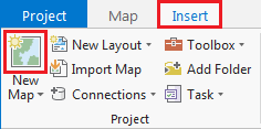
1. On the ribbonRibbon, click the Insert tab.
2. In the Project group, click the New Map button.
   
   
   
   You will notice that a new map view opens in the main section of ArcGIS Pro. The panel on the left side of ArcGIS Pro is called the Contents pane. After creating a new map, the Contents pane now displays the default Map title and automatically adds the Topographic basemap layer to the map. The panel on the right side of ArcGIS Pro is called the Catalog pane. After creating the first map, a new Maps section has been added to the top of the Project tab within the Catalog pane.
   
   
3. In the Catalog pane, click the arrow to expand the Maps section.
   
   
   
   Notice that there is a single map there, named Map. Since most projects will have multiple maps, it is a good idea to name your maps with more descriptive titles.
   
   
4. In the Catalog pane, under the Maps section, right-click Map and select Rename.
5. Type "GISWorkshop" and hit Enter.

...

Any time you create a new project item (such as a map or a layout), spend time adjusting the symbology of your map layers, or are preparing to run a tool, it is a good idea to save your project.

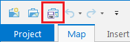
1. Above the ribbonRibbon, on the Quick Access toolbar, click the Save button.
   
   

...

1. In the Contents pane, right-click HST.jpg then click Zoom to Layer.
2. In the Contents pane, click HST.jpg so that is highlighted in light blue. From the ribbonRibbon, click  the Imagery tab and then click the Georeference button. 
   
   
   
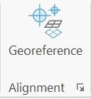
3. Click Add Control Points.
   
   
   
4. Click the top left corner of the HST JPG.
5. Type X : -104.5, Y : 33 and click OK. The x-value is the West coordinate and it is negative because we are in the Western Hemisphere. The y-value is the North coordinate.
6. In the Contents pane, right-click HST and click Zoom to Layer.
7. Repeat steps 5-8 for the bottom right corner of HST, but type X : -103.5, Y : 32. 
8. Repeat steps 5-8 for the bottom left corner of HST but type X : -104.5, Y : 32.
9. Repeat steps 5-8 for the top right corner but type X : -103.5, Y : 33. 
10. From the Georeferencing tab, click Save. 
    
    
    
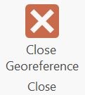
11. Then click Close Georeference.
    
    
    
12. Above the ribbonRibbon, on the Quick Access toolbar, click the Save button.

...

1. In the Catalog pane, expand the Databases section.
2. Right-click PlayMapping.gdb and select New > Feature Class. 
3. Name it "HSTPoints". 
4. Under the Type drop-down box, select Point.
5. Click Next twice. 
6. In the Spatial Reference windowsection, under the Layers section, select the NAD 1927 projection. 
7. ClickNext twice again.
8. Click Finish.
9. If the new feature class did not automatically add iadd to your map: From the Catalog pane in the Databases section, expand PlayMappping.gdb. Right-click HSTPoints and select Add to Current Map. 
10. In the Contents pane, right-click HSTPoints and select Attribute Table. 
11. From the top of the attribute table, click the Add Field button. 
    Image Added
    
12. A new Fields view table pops up. Under appears. In the third row of the Field Name column, add a new name labeled Thickness type "Thickness". 
13. Change the Data Type to Short Integer by clicking the drop-down box then selecting Short. 
14. From the main Ribbon, you will now see you are in the Fields tab. Click , click the Save button on the far right of the Ribbon to save the new field.
15. Close the Fields view table by clicking the X at the top right corner of the table. 
16. From the Ribbon, select the Edit tab.
17. In the Features group, click Create. 
18. A new pane, Create Features, opens on the right side of the screen. Click HSTPoints and select the Point button (first in list). 
19. In the Map view, click to add a point on the topmost left point displayed on the HST.jpg. 
20. In the Attribute Table, a new row has been generated for this newly created point. Click in the Thickness cell for this row and type 7. 
21. Repeat steps 14 and 15 for all points on HST.jpg.
22. From the Ribbon, in the Edit tab, in the Manage Edits group, click Save. Click Yes for the pop-up window. 
23. Close the Create Features pane.
24. Close the Attribute Table. 
25. Above the ribbonRibbon, on the Quick Access toolbar, click the Save button.

...

1. From the Ribbon, click the Analysis tab.
2. In the Geoprocessing group, click the Tools button. A new pane, Geoprocessing, will appear on the right side of the screen. 
3. In the Geoprocessing pane, type Natural Neighbor. 
4. Select Natural Neighbor (Spatial Analyst Tools).
5. Under Input point features, click the drop-down menu and select HSTPoints.
6. Under Z value field, choose Thickness.
7. Under Output raster, change the name to HST_Interp_NN.
8. Click Run.
9. Above the ribbonRibbon, on the Quick Access toolbar, click the Save button.

...

1. Right-click HST_Interp_NN and select Symbology. A new pane, Symbology, will open up on the right side of the screen. From here you can change the symbology settings, which affects how the HST_Interp_NN raster is displayed on the map. Stretched symbology displays continuous raster cell values across a gradual ramp of colors. Classified symbology displays thematic rasters by grouping cell values into classes. 
2. In the Symbology pane, choose Classify from the Primary symbology drop down menu. To change the number or classes, use the drop-down box under Classes. To manually alter the class intervals, double-click the upper values box you would like to edit and enter the new values. To change the color, use the drop-down options under Color Scheme.
3. In the Symbology pane, choose Stretch from the Primary symbology drop down menu. To change the color, use the drop-down options under Color Scheme.
4. Above the ribbonRibbon, on the Quick Access toolbar, click the Save button.

...

1. From the Ribbon, click the Analysis tab.
2. In the Geoprocessing group, click the Tools button. The Geoprocessing pane will appear on the right side of the screen. 
3. In the Geoprocessing pane, type Contour. 
4. Select Contour (Spatial Analyst Tools).
5. From the Input raster drop-down menu, select HST_Interp_NN.
6. Under Output polyline features, name the feature HST_Interp_NN_Contour.
7. Under Contour interval type 10.
8. Leave the Base contour as 0. For other projects you may want to look at the HST_Interp_NN raster range to determine from what value you want the contour intervals to begin.
9. Leave the Z factor as 1. However, if you were using a different thickness than feet, you would want to input the conversion factor here.
10. Click Run.
11. Above the ribbonRibbon, on the Quick Access toolbar, click the Save button.

...

1. From the Ribbon, click the Analysis tab.
2. In the Geoprocessing group, click the Tools button. The Geoprocessing pane will appear on the right side of the screen. 
3. In the Geoprocessing pane, type Excel to Table. 
4. Select Excel to Table (Conversion Tools).
5. For Input Excel File, click the Browse button.
6. On the right side of the Browse window, click Folders.
7. On the left side of the Browse window, double click the PlayMapping folder and choose IGOR_masterlist
8. Under Output Table, name the table GIS_Wells.
9. From the Sheet drop down, choose the GIS_Wells sheet. This ensures that the GIS_Wells sheet will be the data converted from an excel table to a geodatabase table. 
10. Click Run.
11. In the Contents pane, right-click the GIS_Wells table and select Display XY Data.
12. Name the layer GIS_Wells_Pts. 
13. Ensure that the X Field states "longitude" and the Y Field states "latitude". 
14. For Coordinate System, use the dropdown menu to select Current Map [Map]. The coordinate system should now be GCS_North_American_1927. 
15. Click Run.
16. In the Contents pane, rick-click on GIS_Wells_Pts and select Zoom to Layer.
17. Right-click GIS_Wells_Pts and select Label.
18. Right-click GIS_Wells_Pts and select Label Properties. A new pane, Label Class, will open on the right side of the screen.
19. Under the Expression box, clear the current input. 
20. Under the Fields box, double click api_number. The Expression box should now read $feature.api_number.
21. Click Apply.
22. Above the ribbonRibbon, on the Quick Access toolbar, click the Save button.

...

1. In the Catalog pane, expand the PlayMapping project folder.
2. Right-click on geologic_features_poly and select Add to Current Map. 
3. In the Contents pane, right-click on geologic_features_poly and select Symbology. 
4. From the Symbology pane, use the dropdown menu to select Unique Values. Change the Field 1 selection to FEATURE. 
5. From the Color Scheme drop-down, select the color scheme that you would like. 
6. From the Ribbon, click the Analysis tab.
7. In the Geoprocessing group, click the Tools button. The Geoprocessing pane will appear on the right side of the screen. 
8. In the Geoprocessing pane, type Contour. 
9. Select Spatial Join (Analysis Tools).
10. Under Target Features, select GIS_Wells_Pts.
11. Under Join Features, select geologic_features_poly. 
12. Rename the Output Feature Class as GIS_Wells_SpatialJoin. 
13. Retain the default setting of Join_one_to_one for the Join Operation.
14. Retain all other default settings. 
15. Click Run.
16. In the Contents pane, right-click on GIS_Wells_Pts and select Remove.
17. In the Contents pane, click on GIS_Wells_SpatialJoin and rename GIS_Wells. 
18. Above the ribbonRibbon, on the Quick Access toolbar, click the Save button.