Page History

...

1. Using Windows, navigate to your HydrologyLab folder from Lab 1.
2. Double-click the HydrologyLab.aprx ArcGIS Project File.

Creating a new map

Now you will create You will begin by creating a new map for your Lab 2 project. You will begin by opening ArcGIS Pro.

1. On the Standard toolbar, click the Insert tab and click New Map.
   
   
   
   
2. Click the Map title in the table of contents. Rename At the top of the Contents pane, rename the map to "Lab2".

Projecting vector data

Before downloading any new data, you will further process data from Lab 1 in preparation for this lab.

1. On In the catalog Catalog pane, expand the Databases section and the HydrologyLab.gdb file geodatabase.
2. Drag the Watersheds feature class into the Map DisplayLab2 map view.
3. In the Table of Contents pane, double-click the Watersheds layer.
4. In the ‘Layer Properties’ window, click the Source tab.
5. Scroll down and  and expand the Spatial Reference section.
   
   Notice that the layer is in a geographic coordinate system called GCS_North_American_1983. Because NAD 1983, which stands for North American Datum 1983. Because the data has a geographic coordinate system, the coordinates are stored in degrees, which indicate the three-dimensional spherical location of the data on Earth's ellipsoid. Though the data itself is stored in a geographic coordinate system, your computer monitor is flat, so, even though no projection has been defined, the data must be displayed in a particular projection. Whenever ArcMap ArcGIS displays data in a geographic coordinate system, it uses a Plate_Carrée pseudo plate carrée projection, where one degree of latitude by one degree of longitude is represented as a square, rather than a curved trapezoid. In other words, all lines of latitude and longitude are evenly spaced. This type of projection results in increasing stretching in the east-west direction, which increases the farther north or south from the equator you are mapping.
   
   
6. Close the ‘Layer Properties’ window.
   
   Working with geographic coordinate systems is fine for creating purely visual maps, as you did in Lab 1 (though the visual distortion can be disorienting and misleading), but in this lab, you will be calculating areas, distances, and overlaps between features. Such calculations require the three-dimensional coordinates to be projected down onto a two-dimensional plane, so that the coordinates are stored in linear units, such as feet or meters, rather than degrees. In order to facilitate measurements of distance and area, you will now project the Watersheds layer into the State Plane Texas South Central projection which is best suited to mapping the greater Houston region.
   
   
7. In the Analysis tab, click Tools.
8. Under Toolboxes, double-click the Data Management Tools toolbox → Projections and Transformations toolset → Project tool.
9. For ‘Input Dataset or Feature Class’, use the drop-down menu to select Watersheds layer.
   
10. For ‘Output Dataset or Feature Class’, rename “Watersheds_Project” to “Watersheds_StatePlane”, since that is the name of the projection you will be using.
11. Next to the ‘Output Coordinate System’ box, click the Set Coordinate System button.
12. Double-click Projected Coordinate Systems → State Plane → NAD 1983 (2011) (US Feet).
13. Select NAD 1983 StatePlane Texas S Central FIPS 4204 (US Feet) and click OK.
    
    Because both the input and output coordinate systems are based on the NAD 1983 geographic coordinate system, no geographic transformation is required.
    
    
14. Ensure your ‘Project’ window appears as shown below and click Run.
    
15. Close Geoprocessing Pane.
    
    Now that you have the correctly projected layer, you no longer need the original NAD 1983 layer.
    
    
16. Right-click the Watersheds layer and select Remove.
17. Double-click the new Watersheds_StatePlane layer.
    
    Notice that the layer is now in a projected coordinate system, NAD_1983_StatePlane_Texas_South_Central_FIPS_4204_Feet.
    
    
18. Close the ‘Layer Properties’ window.
    

    You may have noticed that the visual appearance of the watersheds did not change in your Map Display, even though you projected them. That is because the data frame takes on the projection of the first layer added to it. Since you first added the original unprojected Watersheds layer into the data frame, which was in NAD 1983, the data frame displays the data in NAD 1983 (or Plate_Carrée). Currently, the projected Watersheds_StatePlane layer is being projected-on-the-fly back into NAD 1983 for visual purposes, so that the two layers are properly aligned in space.

    Move the cursor around the screen and notice that the coordinates in the bottom right corner of the Map Display are shown in decimal degrees. This is another clue that the data frame is still using a geographic coordinate system; however, you would like the data frame to display data using the local Houston projection.
    
    

19. At the top of the Table of Contents pane, right-click the Lab 2 map title and click Properties.

20. Click the Coordinate System tab.
    
    While you could search for or navigate to the State Plane Texas South Central coordinate system, as you did before, in this case, you know that the same coordinate system is already used by the Watersheds_StatePlane layer. In such an instance, it is often easier to import the coordinate system from another known layer, especially if you are not familiar with the hierarchy of the coordinate system folders
    
    

21. On the ‘Coordinate System’ tab toolbar, click the Add Coordinate System button and select Import….
    

22. Double-click the HyrdologyLab geodatabase.
23. Select the Watersheds_StatePlane feature class and click Add.
    
    Notice that the familiar State Plane Texas South Central projection is now listed.
    
    
24. Click OK.
    
    Notice that the watershed boundaries are now more compact in the east-west direction, as expected, because the local projection results in less distortion than the Plate Carrée projection used to represent geographic coordinate systems.
    
    

...

1. Drag the grdn30w095_13 raster into the Map Display.
   
   You will be asked if you would like to create pyramids. Pyramids cache the raster at multiple reduced resolutions, resulting in an increased file size, but better rendering performance in your Map Display. It is normally a good idea to create pyramids, but since you will be processing the corresponding rasters into a new file in the next step, you will not create pyramids at this time.
   
   
2. Repeat Steps 1 and 2 with the grdn30w096_13 and grdn31w096_13 rasters.
   
   Notice that the 1x1 degree tiles appear as angled rectangles, because they are being displayed in the State Plane Texas South Central projection. If the data frame were still in the NAD 1983 geographic coordinate system, the tiles would look like squares. Now you will look up the native coordinate system of the raster files.
   
   
3. In the Table of Contents pane, double-click the grdn31w096_13 layer.
   
   Under the Source tab, scroll down and notice the spatial reference is listed as GCS_North_American_1983. Since this coordinate system is not the same one currently used by the data frame, the raster layer is being projected-on-the-fly into the State Plane Texas South Central projection.

...

1. Close the ‘Layer Properties’ window.
2. Open Tools. Click Toolboxes on the geoprocessing pane.
3. In the Data Management Tools toolbox, click the Raster toolset → Raster Dataset toolset → Mosaic to New Raster tool.
4. For ‘Input Rasters’, select the three 1x1 degree raster layers.
5. For ‘Output Location’, click the Browse button.
6. Select the HydrologyLab geodatabase and click Add.
7. For ‘Raster Dataset Name with Extension’, type “DEMMosaic”.
8. Use the ‘Pixel Type’ drop-down menu to select 32 bit float, since that was the same type stored in the original rasters.
9. For ‘Number of Bands’, type “1”. (The text appears on the right side of the field.)
10. Ensure your ‘Mosaic To New Raster’ appears as shown below and click Run.
    
    The mosaic may take a couple minutes to process. When it is complete, notice there are no longer visual seams between the tiles in the mosaicked raster. Now that you have a single mosaic, you no longer need the three originals tiles.
    
    
11. Remove all three original raster files from the Table of Contents pane.

Projecting raster files

Now you need to project your mosaic into the State Plane Texas South Central projection, so that you can properly calculate spatial statistics based on the data it contains.

...

1. Remove the DEMMosaic layer from the Table of Contents pane.

Clipping raster files

Now you are ready to clip the DEM mosaic to the Buffalo-San Jacinto subbasin.

1. In ArcToolbox, back in the Raster toolset, double-click the Raster Processing toolset and click the Clip (Data Management) tool.
2. For ‘Input Raster’, drag in the DEMStatePlane layer from the Table of Contents pane.
3. For ‘Output Extent’, drag in the Watersheds_StatePlane layer.
4. Check Use Input Features for Clipping Geometry.

...

1. Remove the DEMStatePlane layer from the Table of Contents pane.
2. Turn off the Watersheds_StatePlane layer to view the DEMSubbasin layer.

...

Visually, the meters and feet layers should be identical, but if you look at the layers in the Table of Contents pane, you will notice that the original layer goes from elevations of -8 to 62 meters and the newly calculated layer goes from elevations of -26 to 204 feet.

1. Remove the DEMSubbasin layer from the Table of Contents pane.

Exploring elevation using the raster calculator

...

Typically hillshades are shown beneath transparent layers conveying other information, just to give the map a realistic appearance.

1. In the Table of Contents pane, drag the Hillshade layer beneath the DEMft layer.
2. In the DEMft layer, in the feature-dependent Appearance tab, in the Effects group, slide the transparency to 60%.

...

12. In the HydrologyLab geodatabase, drag the Flowlines feature class into the Map Display.

13. In the Table of Contents pane, drag the Flowlines layer above the DEMft layer, but beneath the Watersheds_StatePlane layer.

...

1. Open Geoprocessing pane by clicking Tools from Analysis tab.
2. In the Spatial Analyst Tools toolbox, double-click the Zonal toolset then click Zonal Statistics as Table tool.
3. For ‘Input raster or feature zone data’, use the drop-down menu to select the Watersheds_StatePlane layer.
4. Use the ‘Zone field’ drop-down menu to select the ‘HU_10_NAME’ field.
5. For ‘Input value raster, select the DEMft layer.
6. For ‘Output table’, rename the table from “ZonalSt_Watersh1” to “WatershedElevation”.
7. Ensure your ‘Zonal Statistics as Table’ window appears as shown and click Run.
   
   

1. In the Table of Contents pane, right-click the WatershedElevation table and select Open.

...

1. Return to ArcGIS Pro.
2. Click the Insert menu and select New Map….
3. Click “Map1” in the contents pane to rename it as “Lab2Precip”. Click Save.
4. Drag Watersheds_Stateplane onto the map display.
5. Click the Geoprocessing tab and search for ‘Excel to Table’.
6. For the Input Excel File, select PrecipStations. Rename the output table PrecipStations.
7. Click Run.
8. In the Table of Contents pane, right-click the PrecipStations table and select Display XY Data.
9. For ‘X Field:’, select the LONGITUDE field.
10. For ‘Y Field:’, select the LATITUDE field.
11. Click the Atlas to the right of the Spatial Reference box.
    
    Because the coordinates are in the form of latitude and longitude in decimal degrees, you know you will need to select a geographic coordinate system, rather than a projected coordinate system.  While the data could theoretically be in any geographic coordinate system, you will select the North American Datum 1983, commonly abbreviated NAD 83, because this is coordinate system of the data provided on the NCDC website.
12. Double-click Geographic Coordinate Systems > North America > USA and Territories.
13. Select NAD 1983 and click OK.
14. Ensure that your window matches that below and click Run.
    
    
    
    The points should now appear on top of the watersheds, though they also extend beyond the watersheds in the Buffalo-San Jacinto subbasin, since we downloaded them for the entire Galveston Bay-San Jacinto subregion.

...

Repeating the technique you learned earlier in this lab to project vector data, project the PrecipStations layer into the State Plane Texas South Central projection.Save the resulting feature class and name it “PrecipStations_StatePlane”. Remove the original PrecipStations layer from the Table of Contents pane.

Create Thiessen polygons

Now you will calculate the mean annual precipitation over each watershed using Thiessen polygons, which associate every cell in the watershed with the nearest rain gage.

1. In the Table of Contents pane, Ctrl-select the PrecipStations_StatePlane and Watersheds_StatePlane layers.
2. Right-click either selected layer and select Zoom To Layers.
3. Open Geoprocessing pane by clicking Tools from Analysis tab.
4. Double-click the Analysis toolbox  then the Proximity toolset then the Create Thiessen Polygons tool.
   
   Before populating the variables in this tool, you will change an Environment setting so that the polygons are calculated for the entire region that you just zoomed to.
   
   
5. At the top of the Geoprocessing window, click the Environments button on the right.
6. For Extent, use the drop-down menu to select Current Display Extent and go back to Parameters.
7. For ‘Input Features’, drag in the PrecipStations_StatePlane layer.
8. For ‘Output Feature Class’, rename the feature class from “PrecipStations_StatePlane_Cr” to “PrecipThiessen”.
9. Use the ‘Output Fields’ drop-down menu to select All fields.
10. Ensure your ‘Create Thiessen Polygons’ window appears as shown below and click Run.
    
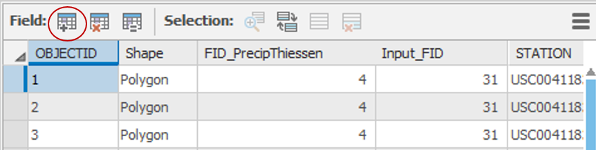
    You will notice that polygons now fill the entire Map Display indicating which areas are closest to which rain gages.
11. Open the PrecipThiessen layer attribute table.
    
    Notice that all of the fields that you originally downloaded from CDO are still included, because you selected to output all fields when running the Create Thiessen Polygons tool. If you do not see all of the same fields, re-run the tool and this time output all fields.
    
    
12. Close the Table.

...

1. In the Analysis Tools toolbox, click the Overlay toolset then the Intersect tool.
2. For ‘Input Features’, drag in the PrecipThiessen and the Watersheds_StatePlane layers.
3. For ‘Output Feature Class’, rename it from “PrecipThiessen_Intersect” to “ThiessenWatershedIntersect”.
4. Ensure your ‘Intersect’ window appears as shown below and click Run.
   
   
5. Remove the PrecipThiessen layer from the Table of Contents pane.
6. Zoom to the ThiessenWatershedIntersect layer.
   
   The resulting layer integrates all of the boundaries from both the Thiessen polygons and the watersheds, limited to the extent of their overlap.
   
   
7. Open the ThiessenWatershedIntersect layer attribute table.
   
   Notice that the original 8 watersheds have now been divided into 42 sections indicating which areas of each watershed are closest to each rain gage. Let P_k denote the annual precipitation associated with each rain gage and A_ik denote the area of the intersected polygon associated with rain gage _k and watershed _i. The area weighted precipitation associated with each watershed is
   
   
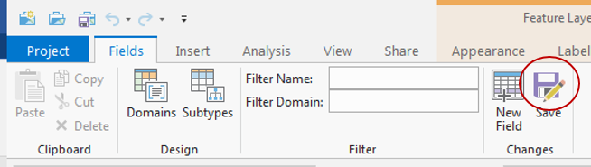
   You will add a new field to the table to calculate the elements of the numerator of the equation.|
   
   
8. Click Add Field… button on top of the table display.
   
   
   
   
9. For ‘Name:’, type “APProd”.
10. Use the ‘Type:’, drop-down menu to select Double and click Save on the Fields tab.
    
    
11. Right-click the APProd field name and select Calculate Field.
12. Using the fields and buttons or by typing, enter “!ANNPRCPHI! * !Shape_Area!”.

13. Ensure your ‘Field Calculator’ appears as shown below and click Run.

    
    The APProd field now contains the numerator values in the equation. You are now ready to summarize the calculated statistics by watershed.

14. Right-click the HU_10_NAME field name and select Summarize….

15. For statistics fields, use the drop-down menu to select the Shape_Area field and select Sum.

16. Select the APProd field and select Sum.
17. For ‘Output Table’, rename the table from “ThiessenWatershedInteract_St” to “WatershedPrecip”.
18. Ensure your ‘Summarize’ window appears as shown below and click Run.
    
    
    The resulting table gives the numerator and denominator in the equation for each watershed.
    
    
19. Open the WatershedPrecip table.

...