Page History

...

1. Leave ‘Output Cell Size’ blank, but­ type “300” for the ‘X’ and ‘Y’.
2. Ensure your Geoprocessing pane appears as shown and click Run.
   Image Removed
   Image Added
   
   

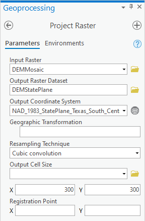
Remember that the data frame was already displaying all layers in State Plane Texas South Central, so you should not notice much of a difference between the two layers, other than that the cell size has increased, meaning the resolution has decreased.

1. Remove the DEMMosaic layer from the Contents pane.

...

Now you are ready to clip the DEM mosaic to the Buffalo-San Jacinto subbasin.

1. At the top left of the Geoprocessing pane, click the Back button.
2. In the search box, type "Clip Raster".
3. Click the Clip Raster toolIn ArcToolbox, back in the Raster toolset, double-click the Raster Processing toolset and click the Clip (Data Management) tool.
4. For ‘Input Raster’, drag in the DEMStatePlane layer from the Contents pane select DEMStatePlane.
5. For ‘Output Extent’, drag in the select Watersheds_StatePlane layer.
6. Check Use Input Features for Clipping Geometry.

...

1. For ‘Output Raster Dataset’, rename the raster from “DEMStatePlane_Clip” to “DEMSubbasin”.
2. Ensure your ‘Clip’ window Geoprocessing pane appears exactly as shown below and click Run.
   Image Removed
   Image Added
   
   
3. In the Contents pane, remove the DEMStatePlane layer.
4. Turn off the Watersheds_StatePlane layer to view the DEMSubbasin layer.

...

Right now, the elevations in the DEM are in units of meters. In order to convert these units into feet, you will use the raster calculator.

1. In At the top left of the Geoprocessing pane, click the Spatial Analyst Tools toolbox, click the Map Algebra toolset, click the Raster Calculator tool the Back button.
2. In the search box, type "Raster Calculator".
3. Click the Raster Calculator tool.
4. In the list of ‘Rasters’, double-click the DEMSubbasin layer.
5. In the calculatorlist of 'Tools', double-click the  the * button symbol.
6. In the equation box, type “3.281”, which is the conversion factor from meters to feet.
7. For ‘Output raster’, rename the raster from “rastercalc” to “DEMft”.
8. Ensure your ‘Raster Calculator’ window appears as shown below and click Run.
   Image Removed
   Image Added
   
   

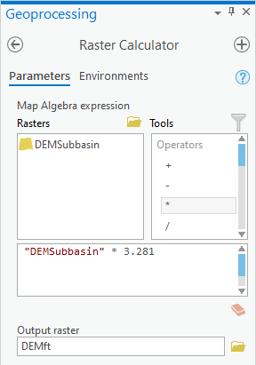
Visually, the meters and feet layers should be identical, but, if you look at the layers in the Contents pane, you will notice that the original layer goes from elevations of -8 to 62 meters and the newly calculated layer goes from elevations of -26 to 204 feet.

1. Remove the DEMSubbasin layer from the Contents pane.

...

Now you will determine which portions of land may be affected by a 15’ storm surge. Obviously, complex inundation models will take more variables into account, but, in this instance, you will simply highlight all the areas of land with an elevation of 15’ or less.

1. Again, go back to In the Raster Calculator tool. Delete , delete the previous expression "DEMSubbasin" * 3.281.
2. In the list of 'Rasters’, double-click the DEMft layer.
3. In the calculator, double-click the <= button.
4. In the equation box, type “15”.
5. For ‘Output raster’, rename the raster from “demftdemft_raster” raster to “Flood15ft”.
6. Ensure your ‘Raster Calculator’ window Geoprocessing pane appears as shown below and click Run.
   
   
   
   
7. RightIn the Contents pane, right-click the Flood15ft layer . Click and click Symbology.
8. In the table of values, right-click the 0 value and click Remove.
   
   
   
   
9. Click the rectangle symbol to the left of the 1 value and select Blue.
   
   
10. Save your project.

Now the cells containing an elevation of 15 feet or less are highlighted on top of the elevation raster.

...

1. For ‘Base contour’, type  “-20”20”.

Since the x,y coordinates are in the units of your State Plane Texas South Central projection, which is feet, and you have also used the Raster Calculator to convert the z units stored within the raster cells to feet, you do not need a custom Z factor.

...

1. In the Geoprocessing pane, search for ‘Table to Excel’.
2. For the Input Table, select ‘WatershedElevation’  WatershedElevation from the drop-down menu.
3. For ‘Output Excel File’, click the Browse button.

If you save this table inside your file geodatabase, you will not be able to open it outside of ArcGIS, so you will instead save it as a text file outside of your file geodatabase.

1. Save the table within the HydrologyLab folder.
2. For ‘Name’, name as “WatershedElevation”“WatershedElevation”.
3. In the ‘Table to Excel’ window, click Run.
4. Close the Table.

Now you will open the exported text file in Excel.

1. Open WatershedElevation.xls in Microsoft Excel.
2. Delete the OBJECTID, ZONE_CODE, COUNT, AREA, and SUM fields.
3. Highlight the minimum and maximum values in each column.

...

1. Click the File menu and select Save As.
2. Navigate to your HydrologyLab folder.
3. For ‘File name:’, type “WatershedElevation” “WatershedElevation”.
4. Use the ‘Save as type:’ drop-down menu to select Excel Workbook (*.xlsx).
5. Click Save and close Excel.

FOR TABLE TO BE TURNED IN

...

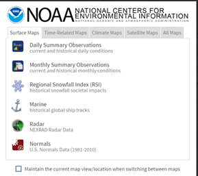
1. In a web browser, go towww.ncdc.noaa.gov/cdo-web/.
2. Click the Mapping Tool tab.
   
   
   
   

You will search for data using the NHD hydrologic units. Previously, you had been working with the Buffalo-San Jacinto subbasin (HUC = 12040104). In this case, you will step up two levels to the Galveston Bay-San Jacinto subregion (HUC = 1204). 

1. On the Surface Maps tab, click Normals.
   
   
   
   
2. In the left sidebar, on the Layers tab, uncheck Daily  Daily Climate Normals, and check Annual  Annual Climate Normals.
3. To the right of Annual Climate Normals, click the Map Tools button.
   
   
   
   
4. In the new ‘ANNUAL CLIMATE NORMALS TOOLS’ window, click Location.
5. Use the drop-down menu to select USGS HUC.
6. Use the ‘Select a HUC type’ drop-down menu to select Subregions (4-digit).
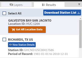
7. Use the ‘Select a HUC’ drop-down menu to select Galveston Bay-San Jacinto.
   
   
   
   
8. ClickZoom to location.
9. The left sidebar switches to the Results tab. Click Get All Location Data.
   
   
   
   
10. For Step 1, select CSV for the output format and click CONTINUE.
    
    
    
11. For ‘Station Detail & Data Flag Options’, check Station name, Geographic location, and Include data flags to include those variables the data table.
    
    
    
    
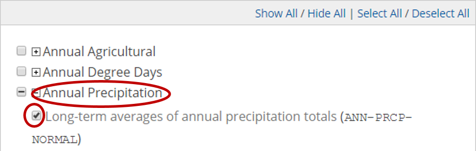
12. For ‘Select data types for custom output’, click the Annual Precipitation category to expand it.
13. Check Long-term averages of annual precipitation totals (ANN-PRCP-NORMAL).
    
    
    
    
14. At the bottom of the window, click CONTINUE.
15. Type your email address twice and click SUBMIT ORDER.

...