In this lab, you will be learning a variety of geoprocessing tools, with a focus on those within the Hydrology toolset. You will start by learning how to recondition a DEM file. You will then calculate flow direction and flow accumulation and learn how to generate drainage lines and catchment basins. Be sure to save your progress often. 

Opening an existing project

1. Using Windows, navigate to your HydrologyLab folder from Labs 1 and 2.
2. Double-click the HydrologyLab.aprx ArcGIS Project File.

Creating a new map

You will begin by creating a new map for Lab 3.

1. On the Standard toolbar, click the Insert tab and click New Map.
   
   
   
   
2. At the top of the Contents pane, rename the map to "Lab3".

Adding data in ArcMap

You will begin by adding the data you previously copied into your geodatabase to the map.

1. In the Catalog pane, expand the Databases section and the HydrologyLab.gdb geodatabase.

Remember that the map view takes on the projection of the first layer added to it. Because you spent time in Lab 2 to ensure that the DEMft raster was in the correct State Plane Texas South Central projection, you will add that layer first, so that your map view will also display in the correct local projection.

1. Drag the DEMft raster into the Lab3 map view.

You can now be sure that the map view will display in the State Plane Texas South Central projection inherited from the DEMft layer. Next you will add the Flowlines layer.

1. In the Catalog pane, drag the Flowlines and Subbasin feature classes into the Lab3 map view.

Though the Flowlines feature class data is still stored in the NAD 1983 geographic coordinate system, in which it was originally provided from NHDPlus, the Flowlines layer is now being projected-on-the-fly into the State Plane Texas South Central projection of the data frame. Remember that projection-on-the-fly may suffice for the purposes of visual display only, but it cannot be used to calculate spatial relationships. Since you will be calculating many such spatial relationships throughout this lab, it is important for all data to be stored in same projection.

Projecting vector data

You will now project the Flowlines layer into the State Plane Texas South Central projection.

1. In the Analysis tab, click the Tools button to open the Geoprocessing pane.
2. In the 'Find Tools' search box, type "project".
3. Click the Project tool.
4. For ‘Input Dataset or Feature Class’, use the drop-down menu to select the Flowlines layer.
   
5. For ‘Output Dataset or Feature Class’, rename “Flowlines_Project” to “Flowelines_StatePlane”, since that is the name of the projection you will be using.
6. For ‘Output Coordinate System’, use the drop-down menu to select the DEMft layer.

Notice that the familiar State Plane Texas South Central projection is now listed. Because both the input and output coordinate systems are based on the NAD 1983 geographic coordinate system, no geographic transformation is required.

1. Ensure your Geoprocessing pane appears as shown below and click Run.
   
   
   
   

Now that you have a correctly projected layer, you no longer need the original NAD 1983 layer.

1. In the Contents pane, right-click the Flowlines layer and select Remove.
2. Repeat the above steps for the Subbasin layer to produce a Subbasin_StatePlane layer.
3. Save your project.
   
   

DEM reconditioning is the process of adjusting a DEM raster so that the elevation values direct drainage towards known vector stream positions, which, in this case, are the flowline features originally obtained from NHDPlus. DEM reconditioning is only suggested when the vector stream information is more reliable than the raster DEM information. The respective accuracy of the DEM and flowlines data has not been assessed in this case, but you will follow the sequence of ArcGIS geoprocessing tools required to carry out reconditioning in order to learn the process.

Converting features to rasters

First, you will convert the vector flowlines into a corresponding raster with exactly the same dimensions (rows, columns, cell size, and alignment) as the DEM raster. Every raster cell intersecting the flowlines will be assigned a value equal to the COMID (Common Identifier, or unique ID) of the intersecting vector flowline and all other raster cells will be assigned a value of NoData.

1. At the top left of the Geoprocessing pane, click the Back button.
2. In the search box, type "feature to raster".
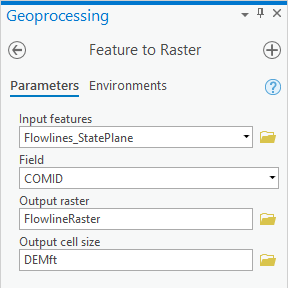
3. Click the Feature to Raster tool.
4. For ‘Input features’, select the Flowlines_StatePlane layer.
5. For ‘Field’, select the COMID field.
6. For ‘Output raster’, rename the raster from “Feature_Flow1” to “FlowlineRaster”.

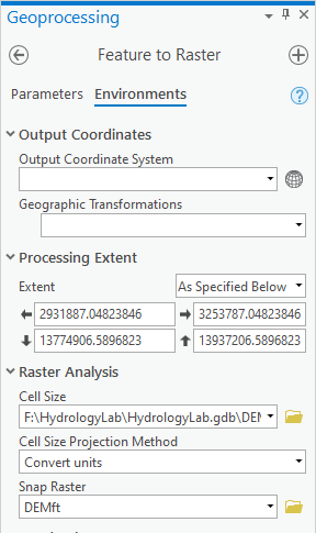
In order to align the cells in this new flowlines raster with the cells in the DEM raster, you will alter the extent, snapping, and cell size using the Environments settings.

1. At the top of the Geoprocessing window, click the Environments tab on the right.
2. Under the 'Processing Extent' section, for 'Extent', select Same As layer: DEMft.

The listed Extent coordinates will be updated based on the geographic extent of the DEMft raster.

1. Under the 'Raster Analysis' section, for ‘Cell Size’, select the Same as layer DEMft.
2. For ‘Snap Raster’, select the DEMft raster.
   
   
   
   
3. At the top of the Geoprocessing window, click the Parameters tab on the left.
4. Ensure your Geoprocessing pane appears as shown below and click Run.
   
   
   
   
5. In the Contents pane, uncheck the Subbasin_StatePlane layer.

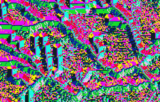
If you zoom in closely, you will notice the raster cells intersecting the Flowlines_StatePlane layer have been added to the FlowlineRaster layer and are assigned a color.

1. Symbolize the FlowlineRaster layer using Unique Values based on the COMID values stored in the Value field, so you can see how the COMID values have been assigned to the cells.
   
   
   
   
2. In the Contents pane, collapse the FlowlineRaster symbology.

Creating a binary raster

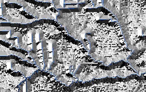
You currently have a raster where each cell contains either the COMID value or the value NoData. NoData cells are transparent, hence you can still see the DEMft layer beneath them. Ideally, you would like a raster where all the flowline cells are assigned a value of 1 to use as a simple flag.

1. Return to the Geoprocessing pane.
2. At the top left of the Geoprocessing pane, click the Back button.
3. In the search box, type "greater".
4. Click the Greater Than (Spatial Analyst Tools) tool.

The Greater Than tool creates a binary raster with a value of 1 anytime the value in the first input raster is greater than the corresponding value in the second input raster. In this case, you would like to assign a value of 1 anytime the COMID value is greater than 1.

1. For ‘Input raster or constant value 1’, select the FlowlineRaster layer.
2. For ‘Input raster or constant value 2’, type “1”.
3. For ‘Output raster’, rename the raster from “Greater_Flow1” to “FlowlineBinary”.
4. Ensure your Geoprocessing pane appears as shown below and click Run.
   
   

The resulting raster assigns each cell a value of 1 when it intersects with a flowline and a value of NoData when it does not intersect a flowline.

Reclassifying a raster

Though you now have a uniform value of 1 to flag the presence of a flowline cell, the remaining cells have a value of NoData, which is not useful for performing mathematical operations across all the cells, so you would like to reassign all cells with a value of NoData to a value of 0.

1. At the top left of the Geoprocessing pane, click the Back button.
2. In the search box, type "reclassify".
3. Click the Reclassify (Spatial Analyst) tool.
4. For ‘Input raster’, select the FlowlineBinary layer.
5. For ‘Reclass field’, select the Value field.

In the ‘Reclassification’ table, you will see a list of old values and new values. You would like to maintain all old values of 1, but you would like to assign all old values of NODATA to a new value of 0.

1. In the New values column, replace the “NODATA” value with a value of “0”.
2. For ‘Output raster’, rename the raster from “Reclass_Flow1” to “Reclassify”.
3. At the top of the Geoprocessing window, click the Environments tab on the right.
4. Under the 'Processing Extent' section, for 'Extent', select Same As layer: DEMft.
5. Under the 'Raster Analysis' section, for ‘Cell Size’, select Same as layer DEMft.
6. For ‘Snap Raster’, select the DEMft raster.
7. At the top of the Geoprocessing window, click the Parameters tab on the left.
8. Ensure your Geoprocessing pane appears as shown below and click Run.
   
   

You will notice that the output raster is a rectangle that encompasses the subbasin, but does not follow its curved boundaries. In the next section, 'Calculating Euclidean distances', you will specify a “mask” that will clip the output raster to the specific geometry of the subbasin. In this case, the null values in the input raster prevented a mask from being an option, so you will retroactively clip the reclassified raster.

1. At the top left of the Geoprocessing pane, click the Back button.
2. In the search box, type "clip".
3. Click the Clip Raster tool.
4. For ‘Input Raster’, select the Reclassify layer.
5. For ‘Output Extent’, select the Subbasin_StatePlane layer.
6. Click Use Input Features for Clipping Geometry.

If this box was not checked, the output would be limited to the rectangular extent encompassing the subbasin, which is the same extent you already have.

1. For ‘Output raster’, rename the raster from Reclassify_Clip to “FlowlineReclass”.
2. Ensure that your Geoprocessing pane appears as shown below and click Run.
   
   

Notice that the extent of the output file is now in the shape of the subbasin.

1. Open the attribute table for the Reclassify layer and note the Count of cells with a value of 0.
2. Now open the attribute table for the FlowlineReclass layer and note the Count of cells with a value of 0.

Notice that, although the visual geometry of the two layers has changed (one is a rectangle, and one is the shape of the subbasin), the total number of cells has not changed. ArcGIS has not automatically updated the attribute table for the clipped raster.

1. At the top left of the Geoprocessing pane, click the Back button.
2. In the search box, type "build raster".
3. Click the Build Raster Attribute Table tool.
4. For 'Input Raster', select the FlowlineReclass layer and click Run.
5. Once again, open the attribute table for the FlowlineReclass layer and note that the number of cells that have been assigned a 0 have decreased to reflect the clipped geometry.
6. Close all attribute tables.
7. In the Contents pane, remove the Reclassify layer.

Now all cells that were previously assigned a value of NoData within the subbasin geometry have been assigned a value of 0.  This will allow you to perform uniform mathematical operations across the entire subbasin in the future.

Calculating Euclidean distances

Next, you will create a new raster where the value of the cell indicates the distance in feet to the nearest flowline.

1. At the top left of the Geoprocessing pane, click the Back button.
2. In the search box, type "euclidean".
3. Click the Euclidean Distance tool.
4. For ‘Input raster or feature source data’, select the Flowlines_StatePlane layer.
5. For ‘Output distance raster’, rename the raster from “EucDist_Flow1” to “FlowlineDistance”.
6. Click the Environments tab.
7. For 'Extent', select Same As layer: DEMft.
8. For ‘Cell Size’, select Same as layer DEMft.
9. For ‘Snap Raster’, select the DEMft raster.

In order to output a raster with the desired geometry of the subbasin, you must apply a mask. Without a mask, the output raster will be a rectangle containing the subbasin geometry, as seen before.

1. For 'Mask’, select the Subbasin_StatePlane layer.
2. Click the Parameters tab.
3. Ensure your Geoprocessing pane appears as shown below and click Run.
   
   
   
   
4. In the Contents pane, right-click the FlowlineDistance layer and select Symbology.
5. For 'Primary symbology', select Classify.
6. For 'Method', select Quantile.
7. For 'Classes', select 5.
   
   
   
   

You should now see cells that vary in color the farther away they are from the nearest flowline.

Performing map algebra

Finally, you are ready to perform the reconditioning step. You can think of this as digging a trench with a funnel-shaped cross-section along each flowline to ensure that water will flow in the intended direction. The math behind this step is explained in the diagram below and all units are in feet, since the State Plane Texas South Central project stores XY coordinates in feet and since you also recalculated the Z elevations in Lab 2 in feet.

1. At the bottom of the Symbology pane, click the Geoprocessing tab..
2. At the top left of the Geoprocessing pane, click the Back button.
3. In the search box, type "calculator".
4. Click the Raster Calculator (Spatial Analyst Tools) tool.

When entering expressions in the raster calculator, your syntax must be exact, so though you could technically type in the equation below, we’d recommend entering everything by clicking the mouse, so you do not get any syntax errors (at least until you’ve learned the proper syntax).

1. By double-clicking the 'Raster' layer names and 'Tools' operations and typing the numbers, enter the following equation: "DEMft" - 30 * "FlowlineReclass" - 0.02 * (1500 - "FlowlineDistance") * ("FlowlineDistance" < 1500).
2. For ‘Output raster’, rename the raster from “demft_raster” to “DEMRecon”.
3. Ensure your Geoprocessing pane appears as shown below and click Run.
   
   
   
   

Notice that the DEMRecon layer looks very similar to the original DEMft. To better understand the difference between the two, you will actually calculate the difference between their corresponding values.

1. In the geoprocessing pane, delete all text from the 'Map Algebra expression' box.
2. Using the same clicking technique as before, enter the following equation: "DEMft” – “DEMRecon”.
3. For ‘Output raster’, rename the raster from DEMRecon to “DEMDiff”.
4. Ensure your Geoprocessing pane appears as shown below and click Run.
   
   
   
   

The DEMDiff layer displays the amount of "earth" that has been removed through the reconditioning process.

You will now undertake a series of geoprocessing steps to understand where water will flow and how much will accumulate. Essentially, you will be learning how to create flowlines and watershed boundaries, similar to those you downloaded from NHDPlus, based on DEM data.

Filling topography sinks

The Fill tool fills sinks in the DEM raster to remove small imperfections in the data. If cells with higher elevations surround a cell, the water gets trapped in that cell and cannot flow. The Fill tool modifies the elevation of the original DEM to eliminate these problems.

1. At the top left of the Geoprocessing pane, click the Back button.
2. In the search box, type "fill".
3. Click the Fill tool.
4. For ‘Input surface raster’, select the DEMRecon layer.
5. For ‘Output surface raster’, rename the raster from “Fill_DEMReco1” to “FIL”.
6. Ensure your Geoprocessing pane appears as shown below and click Run.
   
   

Calculating flow direction

Now you will calculate the cardinal direction in which water from each cell is expected to flow based on the elevations of surrounding cells. Each direction is assigned one of 8 integer values between 1 and 128 as indicated in the illustration below.

1. At the top left of the Geoprocessing pane, click the Back button.
2. In the search box, type "flow".
3. Click the Flow Direction tool.
4. For ‘Input surface raster’, select the FIL layer.
5. For ‘Output flow direction raster’, rename the raster from “FlowDir_FiIL1” to “FDR”.
6. Ensure your Geoprocessing pane appears as shown below and click Run.
   
   
   
   

The result may appear a bit strange at first, due to the color scheme assigned to each cardinal direction.

1. Symbolize the FDR layer using Unique Values with a smooth black and white gradient for the Color Scheme.

You will notice the layer now looks more similar to a hillshade or 3D terrain visualization.

Calculating flow accumulation

Finally, you will calculate flow accumulation in each cell from the cells upstream, as illustrated below. Flow accumulation is dependent on the flow direction you calculated previously.

1. Return to the Geoprocessing pane.
2. At the top left of the Geoprocessing pane, click the Back button.
3. In the search box, type "flow".
4. Click the Flow Accumulation tool.
5. For ‘Input flow direction raster’, select the FDR layer.
6. For ‘Output accumulation raster’, rename the raster from “FlowAcc_FDR1” to “FAC”.
7. Ensure your Geoprocessing pane appears as shown below and click Run.
   
   
   
   
8. In the Contents pane, uncheck the Flowlines_StatePlane layer to better see the FAC layer.
9. Right-click the FAC layer and select Symbology.
10. For ‘Primary symbology’, select Classify.
11. For ‘Method’, select Equal Interval.
12. For ‘Classes’, select 8.
13. In the 'Classes' table, double-click the numbers in the Upper Value column and type the following list: 100, 300, 1000, 3000, 10000, 30000, 100000. (Leave the final max value, 351408 as is.)
14. For ‘Color scheme’, scroll down to the very bottom and select the Yellow-Green-Blue (Continuous) color scheme, as shown below.
    
    

Visually trace along the streams until you find the darkest path exiting the watershed. Notice that, according to the model you have just generated, the Buffalo-San Jacinto basin drains southeast into Galveston Bay.

1. Zoom in to the southeastern outlet point, as indicated below, so that you can see the individual pixels.
   
   

Creating and editing feature classes

You will now create a new point feature class to store the outlet point you just identified.

1. At the bottom of the Symbology pane, click the Catalog tab.
2. Right-click the HydrologyLab.gdb geodatabase and select New > Feature Class.
3. For ‘Name’, type “Outlet”.
4. For ‘Feature Class Type’, select Point.
5. At the bottom, click Next.
6. Click Next again.
7. For 'Current XY', ensure NAD 1983 StatePlane Texas S Central FIPS 4204 (US Feet) is selected.
8. Click Finish.
9. In the Catalog pane, drag the newly created Outlet feature class into the Lab3 map view.
10. On the ribbon, click the Edit tab and click the Create button.
    
    
    
    
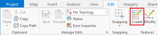
11. On the Create Features pane, select the Outlet layer and click Point button.
    
    
    
    
12. In the map view, click near the center of the outlet pixel to draw a point there.
    
    
    
    
13. On the ribbon, click the Save button.
    
    
    
    
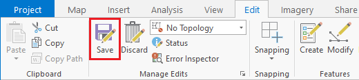
14. When asked if you want to save all edits, click Yes.

Delineating watersheds

Now you will delineate the watershed that flows to the outlet point.

1. At the bottom of the Create Features pane, click the Geoprocessing tab.
2. At the top of the Geoprocessing pane, click the Back button.
3. In the search box, type "watershed".
4. Click the Watershed (Spatial Analyst Tools) tool.
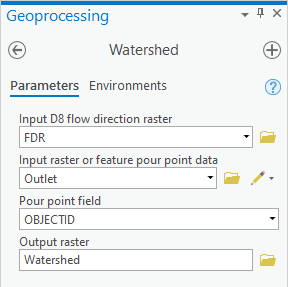
5. For ‘Input D8 flow direction raster’, select the FDR raster.
6. For ‘Input raster or feature pour point data’ select the Outlet layer.
7. For ‘Output raster’, rename the raster from “Watersh_FDR1” to “Watershed”.
8. Ensure your Geoprocessing pane appears as shown below and clickRun.
   
   
   
   
9. In the Contents pane, right-click the Watershed layer and select Zoom To Layer.

You can toggle the Subbasin_StatePlane layer on and off. Notice that the watershed boundary you have created is very close, but does not exactly match the boundaries of the subbasin you were originally provided from NHDPlus.

1. In the Contents pane, turn off all layers beneath the Watershed layer, so that only the cells within the newly defined subbasin are visible.

Delineating streams

Now that you have delineated the subbasin boundaries, you will generate flowlines. The number of flowlines that are generated will depend upon the flow accumulation threshold you select in separating a flowline cell from a non-flowline cell. For the purposes of this lab, you will select a threshold of 3000.

1. At the top left of the Geoprocessing pane, click the Back button.
2. In the search box, type "calculator".
3. Click the Raster Calculator (Spatial Analyst Tools) tool.
4. Using the same clicking technique as before, enter the following equation: ("FAC" > 3000) & ("Watershed" > 0).
5. For ‘Output raster’, rename the raster from “fac_rasterca” to “Streams”.
6. Ensure your Geoprocessing pane appears as shown below and click Run.
   
   
   
   

Again you should have a binary raster, where flowline cells are assigned a value of 1 and all other cells are assigned a value of 0.

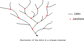
Generating stream links

Now you will separate your entire raster of flowlines into individual flowline segments as illustrated below.

1. At the top left of the Geoprocessing pane, click the Back button.
2. In the search box, type "stream".
3. Click the Stream Link tool.
4. For ‘Input stream raster’, select the Streams raster.
5. For ‘Input flow direction raster’, select the FDR raster.
6. For ‘Output raster’, rename “StreamL_Stre1” to “StreamLinks”.
7. Ensure your Geoprocessing pane appears as shown below and click Run.
   
   
   
   
8. Symbolize the StreamLinks layer using unique values.
9. In the Contents pane, collapse the StreamLinks symbology.

Delineating catchment basins

Now you will delineate the catchment basin associated with each stream link. These catchment basins are similar to the subwatersheds you downloaded from NHDPlus.

1. Return to the Geoprocessing pane.
2. At the top left of the Geoprocessing pane, click the Back button.
3. In the search box, type "watershed".
4. Click the Watershed (Spatial Analyst Tools) tool.
5. For ‘Input D8 flow direction raster’, select the FDR raster.
6. For ‘Input raster or feature pour point data’ select the StreamLinks layer.
7. For ‘Output raster’, rename “Watersh_FDR2” to “CatchmentsRaster”.
8. Ensure your Geoprocessing pane appears as shown below and click Run.
   
   
   
   
9. Symbolize the CatchmentsRaster layer using unique values.
10. In the Contents pane, collapse the CatchmentsRaster symbology.

Converting rasters to features

Now you will convert the CatchmentsRaster raster into a polygon feature class.

1. Return to the Geoprocessing pane.
2. At the top left of the Geoprocessing pane, click the Back button.
3. In the search box, type "raster to polygon".
4. Click the Raster to Polygon tool.
5. For ‘Input raster’, select the CatchmentsRaster layer.
6. For ‘Output polyline features’, rename “RatsterT_Catchme1” to “CatchmentsPoly”.
7. Uncheck Simplify polygons.
8. Ensure your Geoprocessing pane appears as shown below and click Run.
   
   
   
   
9. Symbolize the CatchmentPoly layer using unique values with ID as the value field. Make sure to click the Add all values button.
   
   
   
   
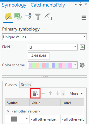
10. In the Contents pane, collapse the CatchmentPoly symbology.

Now you will also convert the raster StreamLinks into a polyline feature class. While you could use the Raster to Polyline tool, you will instead use a tool in the Hydrology toolset, designed specifically for converting raster stream links into polyline features. The difference between the two methods is illustrated below.

1. Return to the Geoprocessing pane.
2. At the top left of the Geoprocessing pane, click the Back button.
3. In the search box, type "stream".
4. Click the Stream to Feature tool.
5. For ‘Input stream raster’, select the StreamLinks raster.
6. For ‘Input flow direction raster’, select the FDR raster.
7. For ‘Output polyline features’, rename the feature class from “StreamT_StreamL1” to “DrainageLines”.
8. Uncheck Simplify polylines.
9. Ensure your Geoprocessing pane appears as shown below and click Run.
   
   
   
   

Calculating Strahler stream order

Now you will use the Strahler method to assign a flow hierarchy to the stream links as illustrated below.

1. At the top left of the Geoprocessing pane, click the Back button.
2. In the search box, type "stream".
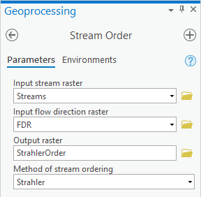
3. Click the Stream Order tool.
4. For ‘Input stream raster’, select the Streams raster.
5. For ‘Input flow direction raster’, select the FDR raster.
6. For ‘Output raster’, rename the raster from “StreamO_Stre1” to “StrahlerOrder”.
7. Ensure your Geoprocessing pane appears as shown below and click Run.
   
   
   
   
8. In the Contents pane, turn off all layers except for the new StrahlerOrder layer, so that its symbology is more apparent.
   
   

Calculating zonal statistics

Now you would like to append this Strahler order to the attribute table of the DrainageLines vector layer, so that you may symbolize that layer using graduated symbols according to the Strahler order number. First, you will need to create a table indicating the Strahler order of each stream.

1. At the top left of the Geoprocessing pane, click the Back button.
2. In the search box, type "zonal statistics".
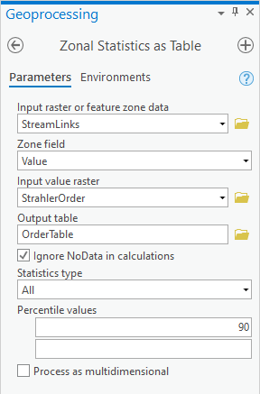
3. Click the Zonal Statistics as Table (Spatial Analyst) tool.
4. For ‘Input raster or feature zone data’, select the StreamLinks layer.
5. For ‘Zone field’, select the Value field.
6. For ‘Input value raster’, select the StrahlerOrder raster.
7. For ‘Output table’, rename the table from “ZonalSt_StreamL1” to “OrderTable”.
8. Ensure your Geoprocessing pane appears as shown below and click Run.
   
   

Adding a new field to an attribute table

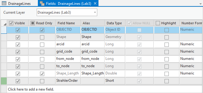
Now you will create a new field in the DrainageLines attribute table to store the Strahler order number.

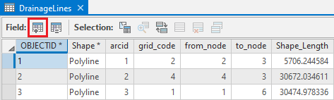
1. Open the DrainageLines attribute table.
2. At the top of the DrainageLines attribute table, click the Add Field button.
   
   
   
   
3. In the bottom row of the table, for ‘ Field Name:’, type “StrahlerOrder”.
4. Use the ‘Data Type:’ drop-down menu to select Short for short integer.
5. Ensure your Fields table view appears as shown below.
   
   
   
   
6. On the ribbon, under the Fields tab, click the Save button.
   
   
   
   
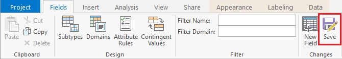
7. Close the Fields table view.

Notice the new StrahlerOrder field has been added to the end of the DrainageLines attribute table. All of the values are currently null, but will later be populated with the Strahler Order integers from the OrderTable.

Joining tables

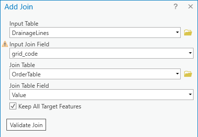
You are now ready to join the OrderTable to the DrainageLines layer based on their common identification fields.

1. At the top right of the DrainageLines attribute table, click the Table Options button and select Joins and Relates > Add Join.
   
   
   
   
2. For ‘Input Join Field’, select the grid_code field.
3. For ‘Join Table’, select the OrderTable table.
4. For ‘Output Join Field’, select the Value field.
5. Ensure that your Add Join window appears as shown below and click OK.
   
   
   
   

Scroll across the table and notice that most of the statistics (Min, Max, Mean, Majority, Minority, Median) are the same and all contain the Strahler order integer, so it doesn’t matter which field you copy, though you will choose the MIN field for this lab.

1. In the attribute table, right-click on the StrahlerOrder field header and select Calculate Field.
2. Scroll down the list of ‘Fields’ and double-click the OrderTable.MIN field and clickOK.
3. Scroll down the newly populated StrahlerOrder field and notice the values of 1, 2, and 3 corresponding to Strahler order value.

Since you have copied the Strahler order into a field in the original DrainageLines attribute table, you no longer need the tabular join.

1. Again, click the Table Options button and select Joins and Relates > Remove All Joins.
2. When asked if you are sure you want to remove all joins, click Yes.
3. Symbolize the DrainageLines layer using graduated symbols based on the StrahlerOrder field.
4. In the Contents pane, turn on only the Outlet, DrainageLines, and CatchmentPoly, layers and turn offall other layers.
   
   

FOR MAP LAYOUT TO BE TURNED IN

Create an 8.5 x 11 layout showing the vector catchment basins along with the stream links symbolized using graduated symbols according to their Strahler order and the outlet point that you used.

1. Create an 8.5 x 11 layout showing the DEMRecon layer.
2. Create an 8.5 x 11 layout showing the vector catchment basins along with the stream links symbolized using graduated symbols according to their Strahler order and the outlet point that you used.