TABLE OF CONTENTS

Obtaining the Tutorial Data

Before beginning the tutorial, you will copy all of the required tutorial data onto your Desktop. There are two ways of obtaining the tutorial data. Option 1 is best if you are completing this tutorial in one of our short courses or from Fondren Library and Option 2 is best if you are completing the tutorial from your own computer.

OPTION 1: Accessing tutorial data from Fondren Library using the gistrain profile

If you are completing this tutorial from a public computer in Fondren Library and are logged on using the gistrain profile, follow the instructions below:

1. On the Desktop, click the File Explorer icon  located on the Windows Taskbar at the bottom left corner of the screen.
2. In the 'File Explorer' window, click This PC on left side panel and then navigate to gisdata (\\file-rnas.rice.edu) (R:) > Short_Courses > HIST207 > HIST207_GDC5 
3. To create a personal copy of the tutorial data, drag the Geoprocessing folder onto the Desktop. 
4. Close all windows.

OPTION 2: Accessing tutorial data online using a personal computer

If you are completing this tutorial from a personal computer, you will need to download the tutorial data online by following the instructions below:

1. Click Geoprocessing.zip above to download the tutorial data.
2. Open the Downloads folder.
3. Right-click Geoprocessing.zip and select Extract All....
4. In the 'Extract Compressed (Zipped) Folders' window, accept the default location into the Downloads folder and click Extract.
5. Drag the unzipped Geoprocessing folder onto your Desktop.
6. Close all windows.

Geoprocessing in ArcGIS Pro

Opening an Existing Project

1. On the Desktop, double-click the Geoprocessing folder.
2. Double-click the Geoprocessing.aprx ArcGIS Project File (blue icon) to open the project in ArcGIS Pro.
   
   
   
   
3. Maximize the ArcGIS Pro application window.

Running Geoprocessing Tools

Geoprocessing tools are used to update and analyze data based on particular criteria. The majority of geoprocessing tools generate a new feature class that differs from the input feature class(es) either in feature geometry or tabular attributes or both. In this tutorial you will use geoprocessing tools to generate information that could be used for a collaboration between the Houston Police Department (HPD) and the Houston Independent School District (HISD).

Merge

The first set of data you will be working with contains the HPD beat boundaries. A beat is the territory and time that a police officer patrols. Though it has been modified for the purposes of this tutorial, the original data was obtained from the City of Houston GIS Database webpage, which is no longer available, but the original data can still be obtained from the GIS/Data Center data collection.

1. In the Catalog pane on the right, expand the Databases folder.
2. Expand the Geoprocessing.gdb geodatabase.
3. Right-click the HPDBeats_North feature class and select Add To New Map.
4. Right-click the HPDBeats_South feature class and select Add To Current Map.

Notice that the police beats in the City of Houston have been divided into two separate feature classes covering the northern and southern portions of the city respectively. You will now examine their attribute tables.

1. In the Contents pane, right-click the HPDBeats_North layer name and select Attribute Table.

Notice that you are provided with both the beat number and the district number for each police beat, and there are 55 beats in the north layer.

1. In the Contents pane, right-click the HPDBeats_South layer name and select Attribute Table.

Notice that the south layer contains 62 beats with the same data fields.

1. Close the NPDBeats_North and NPDBeats_South table views.

At this point, you wish to combine the north and south police beats into a single layer. You will do so using a geoprocessing tool.

1. On the ribbon, click the Analysis tab.
2. On the Analysis tab, within the first Geoprocessing group, click the Tools button.
   
   
   
   

Notice that the Geoprocessing pane has opened on the right as a new tab on top of the Catalog pane. Typically, you would use the 'Find Tools' search box at the top of the Geoprocessing pane to search for the name of the tool you'd like to use, but, at times, especially when learning the software, it can be helpful to view the full hierarchy of all the tools available, because you will often discover related and helpful tools that you didn't know existed and wouldn't know to search for. You might also completely forget the name of a tool, but be able to locate it based on the hierarchy. For these reasons, we will be manually navigating the toolboxes throughout this tutorial. The more typical workflow of searching directly for a specific tool will be covered briefly at the end of the tutorial.

1. At the top of the Geoproccessing pane, click the Toolboxes tab.
2. Click the Data Management Tools toolbox > General toolset > Merge tool.
3. In the upper right corner of the ‘Merge’ tool, hover over the Help button.
   
   

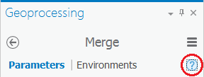
Read the pop-up Merge tool help and review the sample illustration. Notice that this tool merges two like datasets covering different geographic extents together into a single dataset. Clicking on, rather than hovering over, the help button will open the full tool documentation in your default web browser.

1. For ‘Input Datasets’, use the drop-down menu to select the HPDBeats_South layer.

After selecting the HPDBeats_South layer, another drop-down menu appears.

1. Use the second 'Input Datasets' drop-down menu to select the HPDBeats_North layer.

Notice that the when you hover over the 'Output Dataset' field, the file path location defaults to your project geodatabase (C:\Users\gistrain\Desktop\Geoprocessing\Geoprocessing.gdb\HPDBeats_South_Merge).

1. For ‘Output Dataset’, rename the feature class from HPDBeats_South_Merge or HPDBeats_North_Merge to “HPDBeats".
2.  Ensure that your Merge tool Parameters tab appears as shown below and click Run.
   
   

When the tool is finished running, you will see a message at the bottom of the Geoprocessing pane with the name of the tool. A green checkmark indicates that the tool ran successfully.

1. In the Contents pane, right-click the HPDBeats layer name and select Attribute Table.

Scroll down the attribute table and notice that the attributes for both the north and south beats feature classes were preserved and combined into a single table with 117 beats. Since you now have all the beats contained in a single layer, you no longer need the separate layers for the north and south beats.

1. In the Contents pane, right-click the HPDBeats_North layer name and select Remove.
2. In the Contents pane, right-click the HPDBeats_South layer name and select Remove.
3. Above the ribbon, on the Quick Access toolbar, click the Save button.
   
   

Dissolve

Imagine that HPD would like to manage this collaboration based on police district boundaries instead of police beat boundaries. At this point, your HPD layer only displays the police beat boundaries, but its attribute table does tell you the district number corresponding to each beat.

1. Scroll down the HPDBeats table view while observing the values in the District field.

Notice that each district contains many beats. You will now dissolve the police beats based on this District field so that all individual beat boundaries within a single district will be dissolved into a single unified district boundary.

1. Close the HPDBeats table view.
2. At the top of the Geoprocessing pane, click the Back arrow button.
3. Within the already expanded Data Management Tools toolbox, click the Generalization toolset > Dissolve tool.
4. In the upper right corner of the ‘Dissolve’ tool, hover over the Help button.

Read the pop-up Dissolve tool help and review the sample illustration. Notice that this tool dissolves boundaries based on common field values. In this case, you will dissolve the police beat boundaries based on common district values, resulting in a file showing only the larger district boundaries.

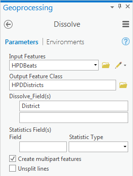
1. For ‘Input Features’, use the drop-down menu to select the HPDBeats layer.
2. For ‘Output Feature Class’, rename the feature class from HPDBeats_Dissolve to “HPDDistricts”.
3. For ‘Dissolve_Field(s)’, use the drop-down menu to select the District field, since this is the field containing the common district values you wish to dissolve on.
4. Ensure that your Dissolve tool Parameters tab appears as shown below, and click Run.
   
   
   
   
5. In the Contents pane, uncheck and recheck the new HPDDistricts layer to toggle it on and off the map and understand the result of the Dissolve tool.
6. In the Contents pane, right-click the HPDDistricts layer name and select Attribute Table.

Notice that only the dissolve field, in this case the District field, was preserved. Because multiple beats were dissolved into each district, it is not possible to retain all of the attributes of each separate beat.

1. Close the HPDDistricts table view.

Since you only need to use the police districts, you may now remove the police beats layer.

1. In the Contents pane, right-click the HPDBeats layer name and select Remove.
2. Above the ribbon, on the Quick Access toolbar, click the Save button.

Clip

Now you will examine the school district boundaries. Though it has been modified for the purposes of this tutorial, the original data was also obtained online from the City of Houston GIS Database webpage, but can now be obtained from the GIS/Data Center data collection.

1. At the bottom of the Geoprocessing pane, click the Catalog tab.
2. Within the Geoprocessing geodatabase, right-click the HISD feature class and select Add To Current Map.

Notice that this feature class displays the boundary of the Houston Independent School District, which can be considered the study area boundary for this project. All of the other data layers you bring into your map document can be clipped to the study area boundary to reduce the size of the files you are working with, which will eliminate visual clutter and allow various processes to run more quickly. First, you will clip the police districts to the study area boundary.

1. At the bottom of the Catalog pane, click the Geoprocessing tab.
2. At the top of the Geoprocessing pane, click the Back arrow button.
3. Click the Data Management Tools toolbox to collapse it.
4. Click the Analysis Tools toolbox > Extract toolset > Clip tool.
5. In the upper right corner of the ‘Clip’ tool, hover over the Help button.

Read the pop-up Clip tool help and review the sample illustration. Notice that this tool clips one dataset to the extent, or shape, of another dataset.

1. For ‘Input Features’, use the drop-down menu to select the HPDDistricts layer.
2. For ‘Clip Features’, use the drop-down menu to select the HISD layer.
3. For ‘Output Feature Class’, rename the feature class from HPDDistricts_Clip to “HPDDistricts_HISD” and click Run.
4. In the Contents pane, uncheck the HPDDistricts layer.

Notice that the resulting HPDDistricts_HISD layer maintains the police district boundaries, but limits the extent of the districts to the extent of the HISD boundary. You no longer need the full extent police districts layer and may remove it.

1. In the Contents pane, right-click the HPDDistricts layer name and select Remove.

You will now work with a dataset containing the locations of all violent crimes (including murder, rape, aggravated assault, and robbery) occurring in 2010, as reported by HPD. Though the data has been pre-processed for this tutorial, the original data tables can be obtained online from the Houston Police Department Crime Statistics webpage at https://www.houstontx.gov/police/cs/crime-stats-archives.htm.

1. At the bottom of the Geoprocessing pane, click the Catalog tab.
2. In the Catalog pane, right-click the HPDCrime2010 feature class and select Add To Current Map.

The crime layer may take a while to load and appear in the map view. You will now clip the crime layer to the study area boundary to reduce the size of the dataset.

1. At the bottom of the Catalog pane, click the Geoprocessing tab.

Notice that the Geoprocessing pane always displays the parameters of the last tool that you ran. Since you want to run the clip tool a second time and will be clipping to the same HISD extent as in the previous run, it is quicker to modify the existing parameters than to click the back arrow and launch the clip tool again from scratch.

1. For ‘Input Features’, use the drop-down menu to select the HPDCrime2010 layer.
2. For ‘Clip Features’, leave the default HISD layer selected from the previous run.
3. For ‘Output Feature Class’, rename the feature class from HPDDistricts_HISD to “HPDCrime2010_HISD” and click Run.

Even though the clip process itself will only take a few seconds, it may again take a couple minutes for the new layer to display on the map view.

1. In the Contents pane, right-click the HISDCrime2010_HISD layer name and select Attribute Table.

Notice that you are provided with the date and hour of the crime, the type of offense, the premise code, the number of offenses, and the approximate address. Since crimes are actually only reported by the block address range, not the exact street address, this address represents the midpoint of the block on which the crime was reported.

1. Close the HISDCrime2010_HISD table view.
2. In the Contents pane, right-click the original HPDCrime2010 layer name and select Remove.
3. In the Contents pane, right-click the HISD layer name and select Zoom To Layer.
4. In the Contents pane, uncheck the HPDCrime2010_HISD and HISD layers, so that only the HPDDistricts_HISD layer is visible.
5. Above the ribbon, on the Quick Access toolbar, click the Save button.

Buffer

The final dataset you will work with contains the locations of all the elementary schools in HISD. Though it has been modified for the purposes of this tutorial, the original data can be obtained online from the Texas Education Agency School District Locator Data Download webpage at http://schoolsdata2-tea-texas.opendata.arcgis.com/

1. At the bottom of the Geoprocessing pane, click the Catalog tab.
2. In the Catalog pane, within the Geoprocessing geodatabase, right-click the HISDElemSchools feature class and select Add To Current Map.
3. In the Contents pane, right-click the HISDElemSchools layer name and select Attribute Table.

Notice that you are provided with the elementary school name, address, and grade range.

1. Close the HISDElemSchools table view.

Now you will create a one-half mile buffer around each school, so that you will later be able to count the number of violent crimes occurring in 2010 within each buffer.

1. At the bottom of the Catalog pane, click the Geoprocessing tab.
2. At the top of the Geoprocessing pane, click the Back arrow button.
3. Within the already expanded Analysis Tools toolbox, click the Proximity toolset > Buffer tool.
4. For ‘Input Features’, use the drop-down menu to select the HISDElemSchools layer.
5. For ‘Output Feature Class’, rename the feature class from HISDElemSchols_Buffer to “HISDElemSchools_HalfMileBuffer”.
6. For ‘Distance [value or field]’, type “0.5” and use the unit drop-down menu to select Miles.
7. Click Run.
8. In the Contents pane, right-click the HISDElemSchools_HalfMileBuffer layer name and select Attribute Table.

Notice that all three fields contained in the original schools point layer (school name, address, and grade range) have been preserved. In addition, a new field has been added stating the radius of the buffer in feet.

1. Close the HISDElemSchools_HalfMileBuffer table view.
2. In the Contents pane, uncheck the HISDElemSchools layer and check the HPDCrime2010_HISD layer.
3. Above the ribbon, on the Quick Access toolbar, click the Save button.

Spatial Join (Points to Polygons)

At this point, you can see all of the violent crime locations, along with the half-mile school buffers, but much of the map is so densely covered with overlapping points that it becomes difficult to tell exactly how many points there are and to see the underlying school buffers. In addition, while you can see the spatial distribution of the points, you are not provided with any sort of useful summary of the data. Performing a spatial join will allow you to discover exactly how many violent crimes occurred within a half mile of each school in 2010.

The goal of performing this spatial join is to add a numeric field to the school buffer attribute table that tells you how many crime points are contained within each school buffer.

1. In the Contents pane, right-click the HISDElemSchools_HalfMileBuffer layer and select Joins and Relates > Spatial Join.

The Spatial Join tool will open within the Geoprocessing pane. For 'Target Features', the HISDElemSchools_HalfMileBuffer is already selected, since that is the layer from which you launched the tool.

1. For ‘Join Features’, use the drop-down menu to select the HPDCrime2010_HISD layer.
2. For ‘Output Feature Class,’ rename the feature class from HISDElemSchools_HalfMileBuff to “HISDElemSchools_HalfMileBuffer_WithCrimeStats".

The 'Field Map of Join Features' describes how the features will be summarized as they are joined. The first half of the list of fields displays the attributes of the school buffer layer, ending with the Shape_Area field. The second half of the list of fields, beginning with the Date field, displays the attributes of the crime layer. A count field indicating how many crime points intersect with each half-mile buffer will automatically be provided. Since many crimes will be appended to each school buffer, it does not make sense to generate summary statistics about the crime fields, because variables like offense type, premise code, and address cannot be averaged. By default, the table would output only the attributes of the first crime encountered within each buffer, which could be very misleading. Therefore, you will remove all the crime attributes from the output fields.

1. Within 'Output Fields', click the Date field.
2. Hold down Shift and click the last Address field, so that all of the crime fields are selected, as shown below.
   
   
   
   
3. Right-click the selected Address field and select Remove.
4. Ensure that your Spatial Join tool Parameters tab appears as shown below and click Run.
   
   
   
   
5. In the Contents pane, right-click the new HISDElemSchools_HalfMileBuffer_WithCrimeStats layer name and select Attribute Table.

Notice the newly added Join_Count field. This field tells you how many crime points are contained within each school buffer. Notice also that only the fields from the schools attribute table have been included in the result, because we removed all the crime fields from the output.

1. Close the HISDElemSchools_HalfMileBuffer_WithCrimeStats table view.

Since the newly joined schools buffer layer contains all of the same information as the original schools buffer layer, plus the new Join_Count field, you no longer need the original buffer layer. Since your crime data has now been summarized, you no longer need the original crime points either.

1. In the Contents pane, right-click the HISDElemSchools_HalfMileBuffer layer name and select Remove.
2. In the Contents pane, right-click the HPDCrime2010_HISD layer name and select Remove.
3. Right-click the HISDElemSchools_HalfMileBuffer_WithCrimeStats layer name and select Symbology.

The Symbology pane has opened on the right as a new tab on top of the Geoprocessing pane.

1. For ‘Symbology', use the drop-down menu to select Graduated Colors.
2. For ‘Field’, use the drop-down menu to select the Join_Count field.
3. Under the 'Upper value' column, click the first upper value and type “25” and press Enter.
4. Click the second upper value and type “50” and press Enter.
5. Click the third upper value and type “100” and press Enter.
6. Click the fourth upper value and type “150” and press Enter.

Leave the fifth upper value as is, since this is the true upper value for the dataset. You can now easily tell which schools have the largest number of violent crimes occurring within a half mile radius.

1. Above the ribbon, on the Quick Access toolbar, click the Save button.

Spatial Join (Polygons to Points)

You now have an attribute table that tells you the number of violent crimes that occurred within one year within a half mile of each school, but you would also like to have a table that tells you in which police district each elementary school lies. To create this table, you will perform another spatial join to add the attributes of the police beat to the back of each school that lies inside it.

1. In the Contents pane, uncheck the HISDElemSchools_HalfMileBuffer_WithCrimeStats layer and check the HISDElemSchools layer.

At this point, only the elementary school point locations and the police district boundaries should be visible.

1. In the Contents pane, right-click the HISDElemSchools layer name and select Attribute Table.

Remember that, at this point, the attribute table only contains the school name, address, and grade range.

1. Close the HISDElemSchools table view.
2. In the Contents pane, right-click the HISDElemSchools layer name and select Joins and Relates > Spatial Join.
3. For ‘Join Features’, use the drop-down box to select the HPDDistricts_HISD layer.
4. For ‘Output Feature Class,’ rename the feature class from HISDElemSchools_SpatialJoin to “HISDElemSchools_WithHPDDistricts".
5. Click Run.

Since each school is entirely within a single district and no data is being summarized, it is okay to leave all of the output fields. The new layer should appear at the top of your Contents pane. 

1. Right-click the new HISDElemSchools_WithHPDDistricts layer name and select Attribute Table.

Notice the newly added District field that tells you which police district each school falls within. Scroll down the table view and notice that five schools do not have a district assigned to them. That is because those schools fall within HISD, but do not fall within the City of Houston police jurisdiction.

1. Close the HISDElemSchools_WithHPDDistricts table view.

Searching for Tools

In this tutorial, you navigated to various geoprocessing tools directly through the Toolbox; however, it is likely that when you go to work on your own, you may not remember exactly where all those tools are located. As long as you can remember the name of the tool or what it does, you can find it using the search function.

1. At the top of the Geoprocessing pane, click the Back arrow button.
2. At the top of the Geoprocessing pane, click the Favorites tab.

This tab shows five commonly used tools, along with all the tools you have run recently and any tools you have marked as a favorite by right-clicking on the tool name and selecting Add To Favorites.

1. In the 'Find Tools' search box, type “clip” and press Enter.
2. Click Clip (Analysis Tools) to open the tool parameters.

Reviewing Tool History

1. At the bottom of the Geoprocessing pane, click the Catalog tab.
2. At the top of the Catalog tab, click the History tab.

Within the history tab, you will see a complete list of all of the tools you have run in order. Double-clicking on any tool in the history will reopen the tool with the exact settings used in that run. Using the History tab is a great way to review previous work for documentation purposes or to rerun a set of tools or slightly modify tool parameters with minimal thought.