...

1. On the Desktop, double-click the Computer icon > gisdata (\\file-rnas.rice.edu) (R:) > Short_Courses > MappingMeasuring_Geographic_Distributions.
2. To create a personal copy of the tutorial data, drag the GeographicDistribution folder onto the Desktop.
3. Close all windows.

...

Opening an Existing Project

1. Within On the GeographicDistributiona folderDesktop, double-click the GeographicDistribution folder.
2. Double-click the GeographicDistribution.aprx project file to open the project in ArcGIS Pro.

...

Sometimes if you want to dig into your spatial dataset, say, find the pattern, or measure the distribution, then the following statistical methods using the ArcGIS tools may work like a charm. The first tool you will learn is the Central Feature tool, which will identify the most centrally located feature in a point, line, or polygon feature class. In this tutorial, we will use the year of 1790, 1870 and 2010 of the States’ Population as the weighting, and we can see the population changing trend across the states.

1790

1. On the right side of the Map Window, in In the Catalog pane on the right, expand the Databases folder.
2. Expand the GeographicDistribution.gdb geodatabase.
3. Right-click the USStatesPopTimeline feature class and selectAdd to New Map.

You may wish to zoom into the continental United States.

1. In the Contents pane to the left of the Map Window, right-click the USStatesPopTimeline layer and selectAttribute Table.

Now you can see that this table has the population data from year 1790 to 2010 (every 10 years) for the total 51states.

Notice that the attribute table contains population data every decade between 1790 and 2010 for each of the 50 states and the District of Columbia. These population counts include only people counted in the official US Census, meaning native populations and populations of territories, among others, are not included.

1. Close the USStatesPopTimeline table viewClose the Attribute Table.

At this point, you wish to find in the year of 1790 determine which state is accessible to the most people in the whole region. You will do so using a spatial statistics tool in the Toolbox.most centrally located when weighted by 1790 population out of all the states admitted as of 1790.

1. On the ribbon, click the Analysis tab.
2. On the Analysis tab, within the first Geoprocessing group, click the Tools button.
   
   Image Added

Notice that the Geoprocessing pane has opened on the right as a new tab on top of the Catalog pane. Typically, you would use the 'Find Tools' search box at the top of the Geoprocessing pane to search for the name of the tool you'd like to use, but, at times, especially when learning the software, it can be helpful to view the full hierarchy of all the tools available, because you will often discover related and helpful tools that you didn't know existed and wouldn't know to search for. You might also completely forget the name of a tool, but be able to locate it based on the hierarchy. For these reasons, we will be manually navigating the toolboxes throughout this tutorial. The more typical workflow of searching directly for a specific tool is covered at the end of the Introduction to Geoprocessing tutorial.

1. At the top of the Geoproccessing pane, click the Toolboxes tab.
2. Click the Spatial Statistics Tools toolbox > Measuring Geographic Distributions toolset > Central Feature toolIn the Analysis tab, click the Tools button. In the Geoprocessing pane to the right of the Map Window, search for ‘Central Feature’. Select Central Feature (Spatial Statistics Tools).
3. For ‘Input Feature Class’, use the drop-down menu, select the USStatesPopTimeline layer.
4. Click the Brows button next to the For ‘Output Feature Class’ menu. Make sure that the file is in the GeographicDistributionData geodatabase and name it USStatesPopTimeline_CentralFeature_1790., rename the feature class from USStatesPopTimeline_CentralF to "USStatesPopTimeline_CF_1790".
5. For In ‘Weight Field,’ use the drop-down menu to select Pop1790.Leave other fields as default the Pop1790 field.
6. Ensure your Geoprocessing pane appears Central Feature tool parameters are configured as shown below . Select Runand click Run.
   
   Image Added

Notice that the output of this tool is the state of Maryland, which was one of the existing features from the original USStatesPopTimeline layer. This state selection makes intuitive sense, since Maryland is located near the center of the original US colonies and is adjacent to the nation's capital.

1870

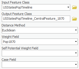
As the Geoprocessing pane doesn’t reset after the tool is completea tool has finished running, it is easy to rerun tools with slightly modified settings. In future versions of ArcGIS Pro, batch processing is also supported, which facilitates multiple runs of the same tool within a single interface.

1. For ‘Output Feature Class’, rename the layer ‘USStatesPopTimelinefeature class "USStatesPopTimeline_CentralFeature_1870’1870".
2. In For ‘Weight Field,’ use the drop-down menu to select Pop1870.Leave other fields as default the Pop1870 field.
3. Ensure your Central Feature window appears tool parameters are configured as shown below . Select and click Run.
   
   Image Added

As we might expect, the 

2010

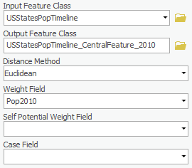
1. In ‘Weight Field,’ select Pop2010.
2. For ‘Output Feature Class’, rename the layer ‘USStatesPopTimeline_CentralFeature_2010’.Leave other fields as default.
3. Ensure your Central Feature window appears tool parameters are configured as shown below . Select and click Run.
   
   Image Added

The Central Feature tool is useful for finding the center when you want to minimize distance (Euclidean or Manhattan distance). If you open the attribute table of each outcome, we could see that from the year of 1790, 1870 to 2010. The center moved from Maryland to Ohio to Illinois.

...

1. In the Geoprocessing pane, click the Back Arrow. In the search bar, search for ‘Mean Center’. Select Mean Center (Spatial Statistics Tools).
2. For the ‘Input Feature Class’ drop-down menu, select USStatesPopTimeline.
3. In ‘Output Feature Class,’ rename the layer ‘USStatesPopTimeline_MeanCenter_1790’.
4. In ‘Weight Field,’ select Pop1790.
5. Leave other fields as default.
6. Ensure your Geoprocessing pane appears Mean Center tool parameters are configured as shown below . Select and click Run.
   
   Image Added

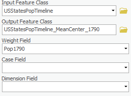
The Mean Center tool creates a new point feature class where each feature represents a mean center (one for each case when a case field is specified). The x and y mean center values, case, and mean dimension field are included as output feature attributes.

...

1. In the Geoprocessing pane, click the Back Arrow. In the search bar, search for ‘Standard Distance’. Select Standard Distance (Spatial Statistics Tools).
2. For the ‘Input Feature Class’ drop-down menu, select USStatesPopTimeline.
3. In ‘Output Feature Class’, rename the layer ‘USStatesPopTimeline_StandardDistance_1790’.
4. In the ‘Circle Size’ drop-down menu, leave it as 1 standard deviation.
5. In ‘Weight Field,’ select Pop1790.
6. Leave other fields as default.
7. Ensure your Standard Distance window appears tool parameters are configured as shown below . Select and click Run.
   
   Image Added

2010

1. Rename the ‘Output Feature Class’ menu ‘USStatesPopTimeline_StandardDistance_2010’.
2. In ‘Weight Field,’ select Pop2010.
3. Leave other fields as default.
4. Ensure your Standard Distance window appears tool parameters are configured as shown below . Select and click Run.
   
   Image Added

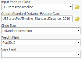
From the output, we can see comparing to 1790, the population distribution of 2010 become less compact.

...

1. In the Geoprocessing pane, click the Back Arrow. In the search bar, search for ‘Directional Distribution. Select Directional Distribution (Standard Deviational Ellipse) (Spatial Statistics Tools).
2. For the ‘Input Feature Class’ drop-down menu, select USStatesPopTimeline.
3. In ‘Output Feature Class’, rename the layer ‘USStatesPopTimeline_DirectionalDistribution1_1790’.
4. In the ‘Circle Size’ drop-down menu, leave it as 1 standard deviation.
5. In ‘Weight Field,’ select Pop1790.
6. Leave other fields as default.
7. Ensure your Standard Distance window appears Directional Distribution tool parameters are configured as shown below . Select and click Run.
   
   Image Added

1790-2SD

1. In the ‘Ellipse Size’ drop-down menu, change to 2 standard deviations.
2. In ‘Weight Field,’ make sure Pop1790 is selected.Leave other fields as default.
3. Ensure your Directional Distribution window appears tool parameters are configured as shown below . Select and click Run.

2010-1SD

1. Rename the ‘Output Feature Class’ ‘USStatesPopTimeline_DirectionalDistribution1_2010’.
2. In ‘Ellipse Size’, select 1 standard deviation.
3. In ‘Weight Field,’ select Pop2010.Leave other fields as default.
4. Ensure your Directional Distribution window appears tool parameters are configured as shown below . Press OKand click Run.

2010-2SD

1. Rename the ‘Output Feature Class’ ‘USStatesPopTimeline_DirectionalDistribution2_2010’.
2. In ‘Ellipse Size,’ change to 2 standard deviations.
3. In ‘Weight Field,’ select Pop2010.Leave other fields as default.
4. Ensure your Directional Distribution window appears tool parameters are configured as shown below . Press OKand click Run.

You can see that the trend from the population distribution of 1790 to 2010. 

Linear

...

Directional Mean

The trend for a set of line features is measured by calculating the average angle of the lines. The statistic used to calculate the trend is known as the directional mean. The Linear Directional Mean tool lets you calculate the mean direction or the mean orientation for a set of line.

...

1. In the ‘Input Feature Class’ drop-down menu, select HoustonFreewaysDissolved.
2. In ‘Output Feature Class’, rename it ‘HoustonFreewaysDissolved_DirectionalMean’.
3. Leave other fields as default.
4. Ensure your Linear Directional Mean pane appears as shown below. Select Run.

Rice Trees

...

1. Click the X on the top right corner of the Geoprocessing pane.
2. In the Catalog pane, expand the Databases folder, and expand the GeographicDistributionData geodatabase. Drag the RiceTrees, RiceTreesCedarElm, and the RiceTreesMediterraneanCypress feature classes into the Map Display.
3. In the Contents pane, right-click on the RiceTrees layer and click Zoom to Layer.
4. In the Analysis tab, click on the Tools button. In the Geoprocessing search bar, search for ‘Directional Distribution’. Select Directional Distribution (Standard Deviational Ellipse) (Spatial Statistics Tools).
5. For the ‘Input Feature Class’ drop-down menu, select RiceTrees.
6. In ‘Output Feature Class’, rename it ‘RiceTrees_DirectionalDistribution’.
7. In ‘Standard Deviation,’ leave as 1 standard deviation.
8. Leave other fields as default.
9. Ensure your Directional Distribution window appears as shown below. Select Run.

CedarElm

1. For the ‘Input Feature Class’ drop-down menu, select RiceTreesCedarElm.
2. In ‘Output Feature Class’, rename it ‘RiceTreesCedarElm_DirectionalDistribution’.
3. In ‘Standard Deviation,’ leave as 1 standard deviation.
4. Leave other fields as default.
5. Ensure your Directional Distribution pane appears as shown below. Select Run.

Mediterranean Cypress

1. For the ‘Input Feature Class’ drop-down menu, select RiceTreesMediterraneanCypress.
2. In ‘Output Feature Class’, rename it ‘RiceTreesMediterraneanCypress_DirectionalDistribution’.
3. In ‘Standard Deviation,’ leave as 1 standard deviation.
4. Leave other fields as default.
5. Ensure your Directional Distribution pane appears as shown below. Select Run.