Page History

...

1. At the top of the Geoprocessing pane, click the Back arrow button.
2. At the top of the Geoprocessing pane, click the Toolboxes tab.
3. Double-click Click the Spatial Analyst Tools toolbox > Interpolation toolset .Click the > IDW (Inverse Distance Weighted) tool.
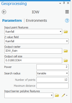
4. For ‘Input point features’, use the drop-down menu to select the Rainfall layer, which contains your rain gauge point locations.
5. For ‘Z value field’, use the drop-down menu to select the Rainfall field that contains the rainfall measurements you wish to interpolate.
6. For ‘Output raster’, rename the exported raster from “Idw_Rainfall1” to “IDW_Rain”.
7.  Ensure that your IDW tool Parameters tab appears as shown below and click Run.
   
   

It will take several seconds for the tool to begin running, at which point you will see the name of the tool along the bottom portion of the Geoprocessing pane. When the tool has finished running, a box will pop up in the same corner with the name of the tool and a green checkmark.

...

You can now see the continuously interpolated raster containing rainfall values that were generated using the data collected at the specific rain gauge points. Notice how this IDW method results in distinct rings around each input data point, because it treats each data point as a local max or min.

1. In the Contents pane, uncheck the IDW_Rain layer.

...

1. At the bottom of the Symbology pane, click the Geoprocessing tab.
2. At the top of the Geoprocessing pane, click the Back arrow button.
3. Within the Interpolation toolset, click the Spline tool.
4. Repeat steps 5-16 above in the Beginning with step 5, repeat all steps in the 'Inverse Distance Weighted Interpolation Method' section on pages 12 and 13above, but rename the output raster output “Spline_Rain”.

Compare the result of the Spline spline interpolation to the result of the IDW interpolation by turning each layer on and off in the Table of Contents pane. Since the layers are transparent, you need to ensure that only one raster is turned on at a time. Notice how the Spline spline interpolation tries to reduce the sharp edges and sudden jumps in data make the data surface as smooth as possible and does not exhibit the distinct rings around the input points, as the IDW method does. The Spline spline interpolation process assumes that, overall, there is a smooth transition in the data and tries to mirror that effect in its output.

1. In the Contents pane, uncheck the Spline_Rain layer and any other raster layers you turned on.

Natural Neighbors Interpolation Method

1. At the top of the Geoprocessing pane, click the Back arrow button.
2. Within the Interpolation toolset, click the Natural Neighbor tool.
3. Repeat steps 5-16 above in the Inverse Distance Weighted Interpolation Method section on pages 12 and 13, but rename the raster output “NN_Rain”.

Compare the result of the Natural Neighbors interpolation to the results of the previous two interpolation methods. Note that it is smooth everywhere except for the distinct highs and lows directly around the data points, though even at the data points it is smoother than in the IDW interpolation method. Note also that the interpolation is limited to the area covered by the input points, rather than a rectangle of the same extent.

1. In the Contents pane, uncheck the NN_Rain layer and any other raster layers you turned on.

TIN Interpolation Method

Using the Create TIN tool, you can create a TIN based on an existing feature class.

Also, notice how the spline method extends any trends that have begun within the region covered by data points way out past the data points, causing extremely high rainfall values in the Gulf and near San Antonio that are far outside the numeric range of the original rain gauge data. The IDW and natural neighbors methods, do not generate values outside the range of the original data.

1. In the Contents pane, uncheck the Spline_Rain layer and any other raster layers you turned on.

Natural Neighbors Interpolation Method

1. At the bottom of the Symbology pane, click the Geoprocessing tab.
2. At the top of the Geoprocessing pane, click the Back arrow button.
3. Within the Interpolation toolset, click the Natural Neighbor tool.
4. Beginning with step 5, repeat all steps in the Inverse Distance Weighted Interpolation Method section above, but rename the raster output “NN_Rain”.

Compare the result of the natural neighbors interpolation to the results of the previous two interpolation methods. It is somewhat in between the two, in that it is smoother than IDW, but not as smooth as spline. While there are not distinct rings around each data point, as there are with IDW, the data points are clearly still creating local highs and lows. Note also that the interpolation is limited to the area covered by the input points, rather than a rectangle of the same extent.

1. In the Contents pane, uncheck the NN_Rain layer and any other raster layers you turned on.

TIN Interpolation Method

Using the Create TIN tool, you can create a TIN based on an existing feature class.

1. At the top of the Geoprocessing pane, click the Back arrow button.
2. Collapse the Spatial Analyst Tools toolbox.
3. Click the 3D Analyst Tools toolbox > Data Management toolset > TIN toolset > Create TIN tool.
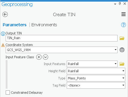
4. For ‘Output TIN’, type “TIN_Rain” and click elsewhere to update the text field.
5. For ‘Coordinate System’, use the drop-down menu to select the Rainfall feature class, which will import the same coordinate system used to map the original latitude and longitude data of the rain gauges.

As you will see in the warning, it is recommended to only create a TIN in a projected coordinate system, rather than a geographic coordinates system. The process of projecting a layer from one coordinate system to another is outside the scope of this course, but is covered in the Introduction to Coordinate Systems and Projections course.

1. For ‘Input Features’, use the drop-down menu to select the Rainfall layer.
2. For ‘Height Field’, use the drop-down menu
3. At the top of the Geoprocessing pane, click the Back arrow button.
4. Collapse the Spatial Analyst Tools toolbox.
5. Double-click the 3D Analyst Tools toolbox > Data Management toolset > TIN toolset.
6. Click the Create TIN tool.
7. For ‘Output TIN’, type “TIN_Rain” and click elsewhere to update the text field.
8. Use the ‘Coordinate System’ drop-down box to select the Rainfall feature class.
9. Use the ‘Input Features’ drop-down box to select the Rainfall feature class.
10. Use the ‘Height Field’ drop-down box to select the Rainfall field.
11. Ensure your ‘Create TIN’ window appears as shown below and click Run.
    Image Removed

This method interpolates the rainfall data points by defining the vertices of each triangle in the TIN and interpolating across each triangle. From here, it is very simple to convert the TIN to a raster, so that it is in the same format as your other interpolation layers.

...