TABLE OF CONTENTS

Obtaining the Tutorial Data

Before beginning the tutorial, you will copy all of the required tutorial data onto your Desktop. Option 1 is best if you are completing this tutorial in one of our short courses or from the GIS/Data Center and Option 2 is best if you are completing the tutorial from your own computer.

OPTION 1: Accessing tutorial data from Fondren Library using the gistrain profile

If you are completing this tutorial from a public computer in Fondren Library and are logged on using the gistrain profile, follow the instructions below:

1. On the Desktop, click the File Explorer icon  located on the Windows Taskbar at the bottom left corner of the screen.
2. In the 'File Explorer' window, click This PC on left side panel and then navigate to GISData (\\smb.rdf.rice.edu\research\FondrenGDC) (O:) > GDCTraining > 1_Short_Courses > Introduction_to_Coordinate_Systems_and_Projections.
3. To create a personal copy of the tutorial data, drag the Projections folder onto the Desktop.
4. Close all windows.

OPTION 2: Accessing tutorial data online using a personal computer

If you are completing this tutorial from a personal computer, you will need to download the tutorial data online by following the instructions below:

1. Click Projections.zip above to download the tutorial data.
2. Open the Downloads folder.
3. Right-click Projections.zip and select Extract All....
4. In the 'Extract Compressed (Zipped) Folders' window, accept the default location into the Downloads folder and click Extract.
5. Drag the unzipped Projections folder onto your Desktop.
6. Close all windows.

Exploring GIS Data in ArcGIS Pro

Opening an Existing Project

1. On the Desktop, double-click the Projections folder.
2. Double-click the Projections.aprx project file to open the project in ArcGIS Pro.

Previewing GIS Data

As a reminder, by default, the far left sidebar is the Contents pane, the central portion of the application window is currently the Catalog view, and the far right sidebar is currently the Catalog pane, but all three show the same list of project items upon first opening a new project.

1. In the Catalog view in the center of the application (not the Catalog pane on the right), double-click the Databases folder.
2. Double-click the Projections.gdb geodatabase.

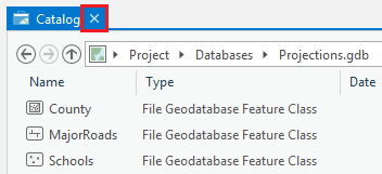
Inside the Projections geodatabase, you will notice three feature classes.

1. Click to select the County feature class.

After selecting a feature class, the right side of the Catalog view now shows the Details panel, which displays the metadata provided for this feature class. In this case, no metadata has been filled out by the data provider.

1. At the bottom of Details panel, click the Preview tab.

This feature class contains a single polygon delineating the boundaries of Harris County. It was obtained from Esri’s Census 2000 TIGER/Line Data website at http://www.esri.com/data/download/census2000-tigerline, which is no longer online, but the same data can be obtained from the United States Census Bureau's TIGER/Line webpage at https://www.census.gov/geo/maps-data/data/tiger-line.html.

1. In the Catalog view, click to select the MajorRoads feature class.

This feature class contains centerlines of all of the major roads within the greater Houston region. It was obtained from the COHGIS 2011 route datasets link on the City of Houston GIS (COHGIS) 2011 Datasets website at http://mycity.houstontx.gov/home/cohgis.html, which is no longer online, but the same data can be obtained from the digital collection in the GIS/Data Center.

1. In the Catalog view, click to select the Schools feature class.

This feature class contains the point locations of all schools in Texas. It was obtained from the Download Schools link on the Texas Education Agency (TEA) Texas School District Locator – Data Download website at http://ritter.tea.state.tx.us/SDL/sdldownload.html, which is no longer online, but the same content can be downloaded at the new Texas Education Agency Public Open Data Site at http://schoolsdata2-tea-texas.opendata.arcgis.com/.

1. In the top left of the main Catalog view, click the small X on the Catalog view tab to close all views.
   
   

Defining Data Projections

All GIS data is created in a particular geographic coordinate system used for mapping locations on a three-dimensional sphere, based on measurements of latitude and longitude. In addition, much GIS data has already been projected onto a two-dimensional plane, based on linear measurements, such as feet or meters. In order for ArcGIS to position a data layer in its proper geographic location, it must be told the proper coordinate system and projection in which the data coordinates were originally created. Otherwise, the data layer can be displayed as an image of sorts, but the image will not necessarily line up spatially with other data layers in the map.

Determining If Layers Are Defined

In some cases, the geographic coordinate system and projection of the data has already been defined in ArcGIS, while, in other cases, you will need to define it yourself based on metadata obtained from the source of the data. First, you will need to determine whether or not each feature class has already been defined.

1. In the Catalog pane on the right, expand the Databases folder.
2. Expand the Projections.gdb geodatabase.

Since the MajorRoads layer is the only one that came from a local agency, it is most likely to have been provided in the ideal projection for this area. Since the map takes on the projection of the first layer that is added to it, we will be sure to add the MajorRoads layer first.

1. Right-click the MajorRoads feature class and select Add to NewMap.

Now you can add any additional layers to your map.

1. Click the County feature class to select it.
2. Hold down Ctrl and click the Schools feature class, so that both feature classes are now selected.
3. Right-click the Schools feature classes and select Add to Current Map.

Now you will investigate whether or not the coordinate systems of the data layers are defined.

1. In the Contents pane on the left, double-click the MajorRoads layer name to open the 'Layer Properties' window.
2. On the left, click the Source tab.
3. Scroll down and expand the Spatial Reference section.
   
   
   
   

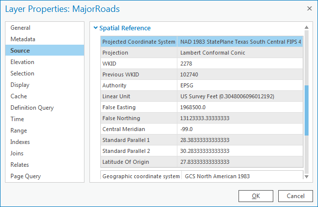
Under the ‘Spatial Reference’ section, scroll down and notice that both a geographic coordinate system and a projection are listed, which indicates that the coordinate system of this feature class has already been defined.

Note that the geographic coordinate system is GCS North American 1983. “GCS” stands for Geographic Coordinate System. This particular coordinate system is more commonly referred to as the North American Datum 1983 or NAD83.

The general type of projection is Lambert Conformal Conic, but its properties (central meridian, standard parallels, latitude of origin, etc.) have been modified to be optimal for South Central Texas. These modifications are saved under the Projected Coordinate System name NAD 1983 StatePlane Texas South Central FIPS 4204 Feet. The State Plane projection system divides each state into multiple planes, or zones, following county boundaries that are suitable for mapping local regions within each state. Houston falls within the South Central plane in Texas.

Finally, notice that the linear unit for this projection is US Survey Feet, which means that the XY coordinates for the data are recorded in feet.

1. In the ‘Layer Properties: MajorRoads’ window, click Cancel.
2. In the Contents pane, double-click the Schools layer name to open the 'Layer Properties' window.
3. On the left, ensure the Source tab is still selected and expand the Spatial Reference section.

Note that the Schools feature class uses the same geographic coordinate system as the MajorRoads feature class: GCS North American 1983. Even the general projection type is the same: Lambert Conformal Conic. However, its properties have been modified to be suitable for all of Texas, rather than just the South Central portion of Texas, so the projected coordinate system name is now Texas Centric Mapping System/Lambert Conformal. The Texas Centric Mapping System is an example of a statewide projection that is suitable for mapping the entire state. Statewide projections are commonly developed for large or elongated states, such as Alaska, California, Michigan, and Texas, which would otherwise be divided into numerous small bands using the State Plane system.

1. In the ‘Layer Properties: Schools’ window, click Cancel.
2. In the Contents pane, double-click the County layer name to open the 'Layer Properties' window.
3. In the left menu, ensure the Source tab is still selected and expand the Spatial Reference section.

Note that the spatial reference is in an unknown coordinate system, meaning that the coordinate system of this feature class has not been defined. In other words, ArcGIS does not know which coordinate system the data was originally created in and, therefore, will probably not be able to accurately line up this data layer with the other data layers. Before you can reliably use this feature class, you will need to define its coordinate system and projection.

1. In the ‘Layer Properties: County’ window, click Cancel.

The geographic coordinate system and projection for each of the three feature classes you investigated are summarized in the table below.

Displaying Undefined Layers

You will now see what happens when you attempt to view an undefined layer in a map. As previously mentioned, the map takes on the coordinate system and projection of the first layer added to it. In this case, since the MajorRoads layer was the first layer added, you expect the map will take on the State Plane Texas South Central projection. To verify this, you will check the coordinate system of the map.

1. Near the top of the Contents pane, double-click Map to open the 'Map Properties' window.
2. On the left, click the Coordinate Systems tab.
   
   

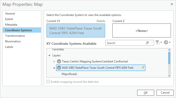
Notice that, indeed, the State Plane Texas South Central projection is listed.

1. In the ‘Map Properties: Map’ window, click Cancel.
2. In the Contents pane, right-click the MajorRoads layer and select Zoom To Layer.

Notice that both the MajorRoads layer and the Schools layer appear to line up properly, even though they have different projections. This is because ArcGIS is able to perform on-the-fly projection, as long as the coordinate systems of both layers are defined. On-the-fly projection means that the Schools layer is being superficially displayed in the State Plane Texas South Central projection of the map, based on calculations performed by ArcGIS; however, the projection of the Schools feature class itself has not been altered from the Texas Centric Mapping System projection.

Though not recommended, on-the-fly projection may be used whenever a visual display of data is all that is required. On-the-fly projection should never be used when attempting to perform calculations between two layers involving measurements of distance or area, as these measurements are most accurate when all data layers are in the same projection.

Now you will see how ArcGIS handles undefined layers.

1. In the Contents pane, right-click the County layer and select Zoom To Layer.

Notice that the County layer does not appear where it should on the map. If you zoom out far enough, you will see that it is in the middle of the Pacific Ocean. This is because ArcGIS does not know where to locate the County layer relative to the other layers, since it is not defined. Instead, ArcGIS does the best it can and treats the coordinates of the County layer as if they were in Texas South Central State Plane coordinates, even though they are not.

1. In the Contents pane, right-click the MajorRoads layer and select Zoom To Layer.

Notice when you move your cursor around the map, the coordinates listed in the bottom of the map view are similar to those shown below, indicating that Houston is located at 95°W, 29°N in NAD 83 in decimal degrees.

While those coordinates are being displayed for general reference purposes, recall that the XY coordinates for data in the State Plane projection are actually stored in feet. You will now change your map view to display units in feet, so that you can see the actual XY coordinates stored in your data.

1. In the Contents pane, double-click Map to open the 'Map Properties' window.
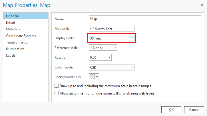
2. On the left, click the General tab.

Notice that the 'Map units' are listed as Foot US, but the 'Display units' are listed as Decimal Degrees. You will now make the display units match the map units.

1. Use the 'Display units' drop-down menu to select US Feet and click OK.
   
   
   
   

Now, notice when you move your cursor around the map, the coordinates listed in the bottom of the map view are similar to those shown below, indicating the location of Houston in the State Plane coordinate system with units of millions of feet.

1. In the Contents pane, right-click the County layer and select Zoom to Layer.

It is evident that both layers are being drawn in the map, but ArcGIS simply does not know how to line them up properly. Notice when you move your cursor around the map now, the coordinates are similar to those shown below, indicating units around 95W and 29E feet.

Whenever you come across X-coordinates between -180 and 180 and Y-coordinates between -90 and 90, you can be fairly sure that they are actually geographic coordinates of latitude and longitude listed in decimal degrees. The fact that you previously observed that Houston is located at 95° W, 29 N° is further confirmation that the county layer was created in a geographic coordinate system, rather than a projection. In this case, ArcGIS is treating these coordinates in decimal degrees as if they were coordinates in feet in the State Plane Texas South Central System, with the end result of locating Harris County near the 0,0 origin of the coordinate system in the middle of the Pacific Ocean within a single square foot.

1. Right-click the MajorRoads layer and select Zoom to Layer.

Whenever you encounter this type of situation, where two layers show up in the Contents pane, but do not line up as you expect them to, you know it is most likely a projection problem.

Determining Projections for Undefined Layers

Of the three feature classes you examined, the County feature class was the only one that was undefined. Since the spatial reference information cannot be located using ArcGIS, you must turn to the source of the data itself. The data was originally downloaded from the following website: http://www.esri.com/data/download/census2000-tigerline, which is no longer available. A screenshot of the metadata provided on that website appears below.

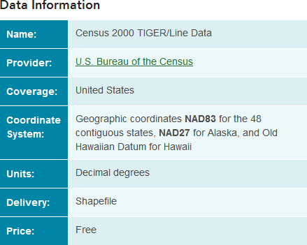
The metadata indicates that you must define the geographic coordinate system for the layer as NAD83, or North American Datum 1983. Fortunately, this is the same geographic coordinate system used by the other two layers. Since no projection is listed, you can assume that the layer has not been projected and was created in a geographic coordinate system only. The fact that the units are listed as decimal degrees further confirms this assumption.

Defining Undefined Layers

Now that you know the geographic coordinate system of the County feature class, you will need to define it, so that ArcGIS knows, as well. Please note that the geographic coordinate system and projection must be defined based on metadata provided from the data source itself. If you cannot locate such metadata, you should contact the provider of the data for the information. You cannot simply guess or decide which projection to use when defining the data (though, occasionally, you may have to resort to educated guesses and trial-and-error when metadata absolutely cannot be tracked down from the data provider.)

1. On the ribbon, click the Analysis tab.
2. In the Geoprocessing group, click the Tools button to open the Geoprocessing pane on the right.
3. In the 'Find Tools' search bar, type "define projection".
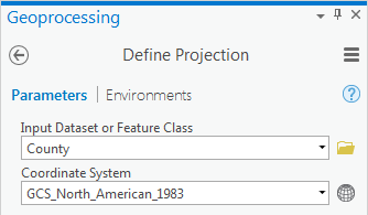
4. Click the Define Projection tool to open it.
5. Use the ‘Input Dataset or Feature Class’ drop-down menu to select County.
6. For the 'Coordinate System', to the right of the drop-down menu, click the Select coordinate system button.
7. In the Coordinate System window, expand Geographic coordinate system > North America > USA and territories.
8. Click NAD 1983 and click OK.
9. Ensure your Geoprocessing pane appears as shown below and click Run at the bottom of the Geoprocessing pane.
   
   

Notice that the County layer has been projected onto the correct location of Harris County.

1. In the Catalog pane, double-click the County layer name.
2. Click the Source tab and expand the Spatial Reference section.

Notice that the geographic coordinate system is now listed, since you have defined the feature class.

1. In the ‘Layer Properties: County’ window, click Cancel.

Projecting Data

If you are only interested in creating a visual map, as you have done now, then relying upon on-the-fly projection will suffice. If, on the other hand, you are interested in performing any sort of calculations between the layers that rely upon distance, area, or spatial overlap, then it is recommended that you use the same projection for all layers. In addition, you can only measure linear distances in a projected coordinate system, not in a geographic coordinate system, so the County layer would need to be projected anyway, before any sort of measurements could be made.

Selecting a Map Projection

Now that all of your data has been defined, you can transform all the feature classes into a common projection. Unlike the process of defining data, where there is only one projection you can use (the one specified in the metadata), when projecting data, you can select whichever projection best suites your particular study area and research question measurement types. Since your data focuses on the Houston region, the State Plane Texas South Central projection would be suitable.

Determining Which Layers to Project

The State Plane Texas South Central projection has been selected for the final map projection.  All layers that are not currently in that projection will need to be re-projected, such as the County and Schools feature classes. All layers that are already in the final projection can be left as is and do not need to be re-projected, such as the MajorRoads feature class.

Projecting Layers

1. At the top of the Geoprocessing pane, click the Back arrow.
2. In the 'Find Tools' search bar, type ‘project’.
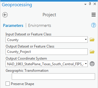
3. Click the Project tool to open it.
4. For 'Input Dataset or Feature Class', use the drop-down menu to select the County layer.

Note that the output dataset is saved to the same geodatabase as the input dataset and the name of the output feature class has the suffix “_Project” appended to the end of the original input feature class name to indicate which tool was used to produce that feature class.

1. For ‘Output Coordinate System’, use the drop-down menu to select the MajorRoads layer.

Notice that the NAD 1983 State Plane Texas South Central projection has now been imported from the MajorRoads layer. While you could have again navigated to the projection yourself, in this case, you know that the same coordinate system is already used by the MajorRoads layer. In such an instance, it is easier to import the coordinate system from another layer, especially if you are not familiar with where the coordinate system of interest is stored in the overall hierarchy.

1. Ensure that your Geoprocessing pane appears as shown below and click Run.
   
   

When previously defining a layer, you simply updated the metadata attached to that layer to include the known coordinate system and projection. When projecting a layer, you have actually created a second copy of the data in the new coordinate system. The original layer stays in the native coordinate system and the new layer is converted to the desired coordinate system.

1. In the Catalog pane, double-click the County_Project layer name.
2. On the left, ensure to the Source tab is still selected and expand the Spatial Reference section.

Note that the geographic coordinate system is still GCS North American 1983 and that the new coordinate system is NAD 1983 StatePlane Texas South Central FIPS 4204 Feet.

1. In the ‘Layer Properties: County_Project’ window, click Cancel.

You will now repeat the same process to re-project the Schools feature class from the Texas Statewide Mapping System projection into the State Plane Texas South Central projection.

1. Repeat all steps in the 'Projecting Layers' section with the Schools layer. When your Geoprocessing pane appears as shown below, select Run.
   
   
   
   

All of your layers have now been projected into the State Plane Texas South Central projection.

1. In the Contents pane, right-click the Schools layer and select Remove.
2. In the Contents pane, right-click the County layer and select Remove.

Since all layers in your data frame are now in the same projection, you could proceed to make accurate calculations of distance and area between the layers.