...
- At the top of the Geoproccessing pane, click the Toolboxes tab.
- Click the Spatial Statistics Tools toolbox > Analyzing Patterns toolset > Spatial Autocorrelation (Global Moran's I) tool.
- In the upper right corner of the ‘Spatial Autocorrelation’ tool, hover over the Help ? button.
(Help)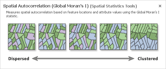
The Spatial Autocorrelation tool evaluates whether data is clustered, dispersed, or randomly distributed based on both feature locations and feature values simultaneously.
...
- Hover over the Completed with warnings message to display the tool parameters and messages.
(Pic ToolMessages)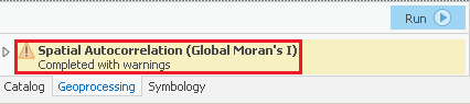
Under the lower 'Messages' section, notice that the warning message indicates that the neighborhood search distance used in the analysis was 38893 feet. Since the distance threshold does impact the statistical results, it is important to make note of it. You will learn more about the impact of the distance threshold later on. While the Moran's Index and z-score are also displayed in the messages, they are easier to interpret in the context of the report.
- Within the 'Spatial Autocorrelation Parameters and Messages' pop-up window, click the Report File hyperlink to open the report in your default web browser.
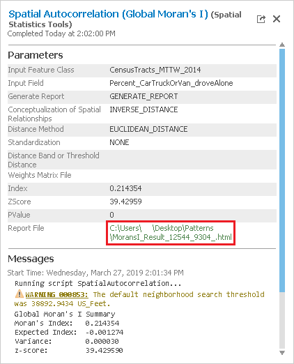
In the top left, notice that the z-score is 39.43. In the top right, notice that any z-score larger than 2.58 has less than 1% chance of occuring randomly. In the center section is the normal distribution curve and a dotted line illustrating where the z-score for this analysis is located on that curve. It also illustrates that a positive z-score indicates that the data is clustered, while a negative z-score would indicate that the data is dispersed. Below the diagram is a helpful summary sentence, "Give the z-score of 39.43, there is a less than 1% likelihood that this clustered pattern could be the result of random chance." Because the z-score is more than an order of magnitude larger than 2.58, you will notice in the top left that the p-value is actually 0.00, which means there is no chance that this pattern is random. While simply knowing that the percentages of people who drove alone to work are highly clustered might not provide you with actionable knowledge, what this result does indicate is that there is a strong pattern present, which is worth investigating further. Because you know your data displays strong clustering, you can now ask more interesting questions. Is it the high or low percentages of commuters driving alone that are clustered? Where are they clustered? You will see find that all of the spatial statistics tools build upon each other to provide additional knowledge.
...