...

1. In the ‘Licensing’ window, select Single Use License for License Type, as shown on the following page, once it finishes loading and click OK.
   
2. In the ‘ArcGIS Pro’ window, select Blank.
   Image Modified

1. In the ‘Create a New Project’ window, type HydrologyLab as Name and click the icon to navigate to the HydrologyLab folder created. Uncheck Create a new folder for this project. Click OK.
   Image Modified

1. In the Insert tab, click ‘New Map’.
   Image Modified

1. On Contents pane, clickMap name to rename it from Map to Lab1.
   Image Modified

...

1. In a web browser, go to www.arcgis.com.
2. In the search box in the top right of the website, type “NFIE-Geo Regions”.
3. Click to Open the NFIE-Geo Regions web map.
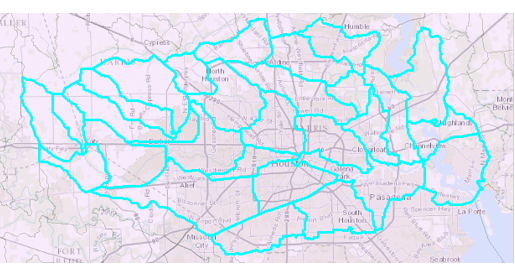
4. On the map, click to select the Texas-Gulf region, which encompasses Houston.
5. Click More info.
6. In the Content section, right-click the NFIEGeo_12.gdb.zip file and select Download.
   Image Modified

1. Navigate to the location where the zipped file has been downloaded.
2. Right-click the downloaded NFIEGeo_12.gdb.zip file and select Extract All….
3. In the ‘Extract Compressed (Zipped) Folders window, click Extract.
4. In the new extracted folder window that opens, right-click the extracted NFIEGeo_12.gdb folder and select and Copy.
5. Navigate back to your HydrologyLab folder.
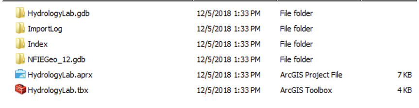
6. Paste the NFIEGeo_12.gdb folder directly inside your HydrologyLab folder. Do NOT paste them inside the Hydrologylab.gdb geodatabase.
7. Ensure that your HydrologyLab folder appears as shown below.
   Image Modified

1. Return to ArcGIS Pro.

Unfortunately, any changes you make to files outside of ArcGIS Pro are not automatically reflected inside ArcGIS Pro. Since you just added new files to your HydrologyLab folder, you will need to refresh your HydrologyLab folder in order for them to appear.

...

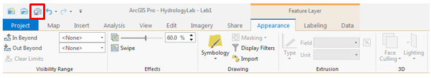
1. On the Standard toolbar, click the Basemap button.
   Image Modified

1. In the ‘Basemap’ window, select the Topographic basemap.

...

1. In the Table of Contents, click and select the Subwatershed layer. Click Appearance Tab.
   Image Modified

1. Under effects, type “60” to change the transparency of the layer.

...

1. On the Map tab, select Select by Attributes….
   Image Modified

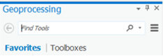
1. In the Geoprocessing pane, use ‘Layer Name or Table View’ drop-down menu to selectSubwatershed.
2. Use the ‘Selection Type’ drop-down menu to select New selection.
3. Click Add Clause.
   Image Modified

1. Select Values.

A list of all values stored in the HUC_8 field will appear in the box on the right.

1. Select Subwatershed, and is equal to, in the first two fields.
2. Type ‘12040104’ in the last field.
3. Verify that your ‘Select By Attributes’ pane appears as shown on the following page and click Add.
   Image Modified

1. Click Run.
2. In the Table of Contents, right-click the Subwatershed layer and select Selection -> Zoom To Selection.
   Image Modified

Exporting selected features

...

1. For ‘Output feature class:’, rename “Subwatershed_CopyFeatures” to “SubwatershedsNew”.
2. Ensure your ‘Copy Features’ window appears as shown below and click Run.
   Image Modified

Since you’ve exported the particular subwatersheds of interest, you may now remove the master subwatersheds layer from your map document.

...

1. On the Standard toolbar, click the Save button.
   Image Modified

At the top of the Table of Contents window, notice that the leftmost List By Drawing Order button is currently selected.

1. At the top of the Table of Contents, click the List By Source button.
   Image Modified

The Source tab displays the full file path locations of all the data layers referenced in your map document. By default, the map document will store this full file path to all of your data files.

...

1. On the Map tab, click the Analysis tab and select the Tools.
2. On the search bar, type Dissolve and press Enter. Double-click Dissolve (Data Management Tools).
   Image Modified

1. In the top right corner of the ‘Dissolve’ window, click question mark icon.

...

1. For ‘Input Features’, drag in the SubwatershedsNew layer from the Table of Contents.
2. For ‘Output Feature Class’, rename the feature class from “SubwatershedsNew_Dissolve” to “Subbasin[g1] ”.
3. For ‘Dissolve_Field(s)’, select the HUC_8 field, since this is the field containing the common subbasin value you wish to dissolve on.
4. Ensure your ‘Dissolve’ window appears as shown below, and click Run.
   Image Modified

1. In the Table of Contents, toggle the new Subbasin layer off and on to get a better idea of the result of the Dissolve tool.
2. In the Table of Contents, right-click the Subbasin layer and select Attribute Table.

...

1. In the Table of Contents, click the rectangle symbol beneath the Subbasin layer name to open the ‘Symbology’ tab.
2. On the top of the tab, click Properties.
   Image Modified

1.  For ‘Color:’, use the drop-down menu to select No Color.
2. For ‘Outline Color:’, used the drop-down menu to select Black.
3. For ‘Outline Width:’, type “2”.
4. Click Apply.

...

While you could have also dissolved using the HU_10 field, the watershed name is probably more meaningful to you than the HU_10 code.
Image Modified

Notice that the subwatersheds from the previous layer have now been grouped into 7 watersheds within the Buffalo-San Jacinto subbasin.

1. As before, apply 60% transparency to the Watersheds layer.
2. Make sure that the Watersheds layer is selected in Contents and click Labeling under Feature Layer tab on the main tab display.
3. Select HU_10_Name in the Field drop-down menu.
4. Click the Label icon to turn on the labels.
   Image Modified

Depending on your screen size, you may notice the easternmost watershed does not get labeled if there is not adequate space for the required text. This could be adjusted using advanced labeling techniques, but you will leave the map as is.

...

1. On the main tab, click Insert -> New Layout -> ANSI Landscape -> Letter.
2. Click Insert tab and click Map Frame.
3. Select the Lab1 map under Map.
   Image Modified

1. Select Layout tab and click Activate.
2. Right-click Watersheds layer and click Zoom to Layer.
3. Select Layout tab and click Close Activation.
   Image Modified

Using techniques you learned last week, create a suitable map, as described for the map layout to be turned in below. If you would like to orient the page in landscape, open the ‘Page and Print Setup’ window from the File menu. All map elements, such as text, legends, north arrows, and scale bars can be added to the layout from the Insert menu.

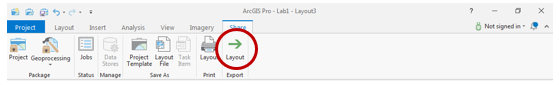
1. Select Share Tab and click Export Layout.
   Image Modified

1. Save your map document.

FOR MAP LAYOUT TO BE TURNED IN

...

1. Ensure your ‘Select by Location’ window appears as shown and click Run.
   Image Modified

All of the flowlines catchment areas that are within the subbasin are now selected.

...

1. If necessary, go to the Catalog window and click Layouts on top of the map display to get in layout mode.
2. Click the Insert tab. Select the drop down menu of Text and click Rectangle.
   Image Modified

1. Drag a rectangle on your map layout to insert a rectangle text element.

...

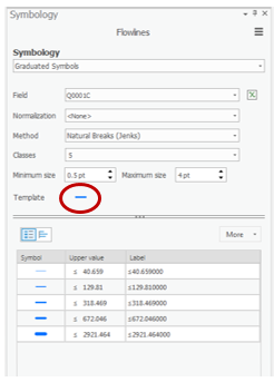
1. Open the Flowlines Symbology tab.
2. Use Symbology drop down menu to select Graduated symbols.
3. Use the ‘Field’ drop-down menu to select the Q0001C field, which contains the mean annual flow.
4. Click the line next to Template to change the symbology of your flowlines.
   Image Modified

1. Save your map document.

FOR MAP LAYOUT TO BE TURNED IN

...

1. In the table of contents, check the StreamGages layer which you brought in at the beginning with the Geographic feature dataset from the NFIEGeo_12 Geodatabase.
2. On the Main menu, click Select By Location….
3. For ‘Input Feature Layer’, check the StreamGage layer.
4. For ‘Relationship’, use the drop-down menu to select within.
5. For ‘Selecting Features’, use the drop-down menu to select Subbasin.
6. Ensure your ‘Select by Location’ window appears as shown and click Run.
   Image Modified

All of the stream gages that are within the subbasin are now selected.

...

1. Scroll down and click the result SSURGO Downloader.
   Image Modified

1. On the right hand side of the page click View Application.
   Image Modified

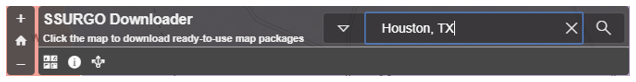
1. In the search bar in the top right corner, type Houston, TX.
   Image Modified

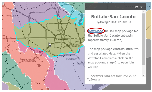
1. Click in the Buffalo-San Jacinto subbasin to select it and click the Download link.
   Image Modified

1. Right-click on your downloaded BuffaloSanJacinto_12040104.mpk file and select Show in folder. Copy its file path location.
2. Open ArcGIS Pro, click Insert tab and select Import Map.
   
3. Paste the file path location to import window. Press Enter. Select BuffaloSanJacinto_12040104.mpk file.
4. Click OK.
   Image Modified

A map package (.mpk), contains both a map document (.mxd) and all data layers referenced by that map document. A new instance of ArcMap will open showing the different soil classes within the subbasin.

...

1. On the Map tab, click the Analysis tab and select the Tools.
2. On the search bar, type Clip and press Enter. Click Clip (Analysis Tools).
   Image Modified

Read the ‘Clip’ window help and review the sample illustration. Notice that this tool clips one dataset to the extent, or shape, of another dataset.

...

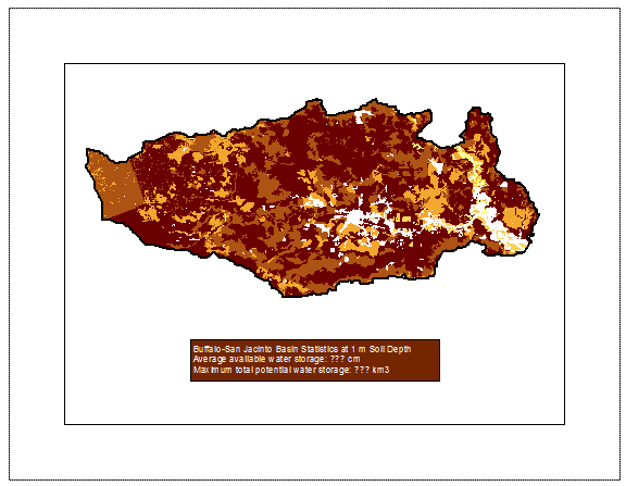
1. What is the average available water storage (cm) in the Buffalo-San Jacinto subbasin?
2. Based on your previous calculation of the area of the subbasin in km², what volume of water (km³) could potentially be stored in the top 1 m of soil in the Buffalo-San Jacinto subbasin if the soil were fully saturated with water?
   Image Modified

Exporting map documents

1. To export both your Lab1Hydrology and Lab1Soils map documents, open each of them in turn and click the Project menu and select Export Map….
2. Navigate to your HydrologyLab folder.
3. Use the ‘Save as type:’ drop-down menu to select PDF.
4. Click Save.
5. Print both map PDFs to turn in

...