In this lab, you will practice downloading, manipulating, mapping, and analyzing publicly available hydrology data from a variety of online websites to study the Buffalo-San Jacinto watershed subbasin, which encompasses the greater Houston region. Specifically, you will work with watershed and flowline data from the National Flood Interoperability Experiment (NFIE), stream gage data from the National Water Information System (NWIS), and soils data from the Soil Survey Geographic Database (SSURGO).
Part 1: Setting Up a GIS Project
Creating a new project folder
First, you will need to establish a project folder, where you will store all of the files associated with this lab assignment. When working in a public computer lab environment, we recommend saving your work on an external USB drive. For the purposes of illustration throughout these lab instructions, the project folder will be located directly on a USB drive, which is mapped as the F: drive, though your USB drive letter may vary. If you wish to nest your project folder inside other folders within the file organization scheme on your USB drive, ensure that no spaces or special characters are used anywhere along the entire file path of your project folder.
- Using Windows Explorer, navigate to the location where you would like to locate your project folder (likely the E: or F: drive).
- Create a new folder inside your selected location and name it “HydrologyLab”. Remember not to use any spaces. Note the full file path of your HydrologyLab folder.
Connecting to a project folder
Now that you have created a project folder for this lab, you will need to connect to it in the ArcGIS for Desktop environment.
...
- On Contents pane, clickMap name to rename it from Map to Lab1.

Part 2: Mapping Watershed Data
Downloading NFIE data
Your project folder and geodatabase have been created, so you are ready to download your first set of online GIS data. You will start by downloading data from the National Flood Interoperability Experiment (NFIE), which is searchable on the ArcGIS Online platform.
...
- In the Catalog Pane on the right of the map display, expand Folders , right-click your HydrologyLab folder and select Refresh.
- Expand the NFIEGeo_12 geodatabase and the Geographic feature dataset to preview what layers it contains .
- Drag the Geographic feature dataset on Catalog Pane into the Map Display.
Adding feature data in ArcMap
If you ever close the Catalog window, causing the Catalog tab to disappear, you can reopen it by clicking the Catalog button on the Standard toolbar or by clicking the Windows menu and selecting Catalog.
...
- Close the attribute table.
Adding an online basemap
First, you would like to identify the subwatersheds within the greater Houston region, but without any additional reference layers regarding streets or administrative boundaries, this would be very difficult to do. Fortunately, you can utilize various basemaps of the world hosted online by Esri, rather than having to obtain all of the GIS reference layers yourself. Because these basemaps are being hosted online, they cannot be edited and can sometimes be slow to load.
...
Now the basemap should be visible beneath the subwatersheds.
Identifying features
Ultimately, you want to select all of the subwatersheds that lie within the Buffalo-San Jacinto subbasin in which Houston is located, but first you will need to look up the HUC-8 code corresponding to this subbasin.
...
In the ‘Identify’ window, notice that the HUC_8 field contains the code 12040104, which corresponds to the Buffalo-San Jacinto subbasin. The first two digits (12) stand for the region (Texas-Gulf Region). The next two digits (1204) stand for the subregion (Galveston Bay-San Jacinto). The next two digits (120401) stand for the basin (San Jacinto). The last two digits (12040104) stand for the subbasin (Buffalo-San Jacinto). The additional two digits added to create the HUC-10 and HUC-12 codes stand for the watershed and subwatershed, respectively.
- Close the pop-up window.
Performing an attribute query
Now you are ready to perform an attribute query to select all of the subwatersheds within the Buffalo-San Jacinto subbasin (HUC-8 = 12040104).
...
- Click Run.
- In the Table of Contents, right-click the Subwatershed layer and select Selection -> Zoom To Selection.
Exporting selected features
Now that the Buffalo-San Jacinto subwatersheds have been selected, they can be exported into a separate layer stored in your HydrologyLab geodatabase.
...
- Right-click the Subwatershed layer and select Remove.
Saving ArcGIS projects
At this point, it is a good idea to save your map document and to continue saving regularly.
...
- At the top of the Table of Contents, click the List By Drawing Order button to return to the list of data layers.
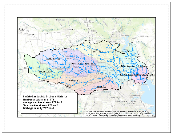
Geoprocessing: Dissolving features
Now you would like to highlight the boundary of the entire Buffalo-San Jacinto subbasin, but if you tried to change the outline of the current subwatersheds layer, it would change the outline around all subwatersheds. Instead, you will dissolve all the subwatersheds into a single subbasin feature stored in a new feature class inside your HydrologyLab geodatabase.
...
- In the Table of Contents, uncheck the original SubwatershedsNew layer.
- In the Table of Contents, drag the Subbasin layer above the Watersheds layer, so it is fully visible again.
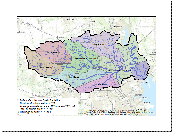
Symbolizing features by categories using unique values
Now that you have generated the watershed features within the Buffalo-San Jacinto subbasin, you will symbolize them based on their HUC-10 watershed name.
...
Depending on your screen size, you may notice the easternmost watershed does not get labeled if there is not adequate space for the required text. This could be adjusted using advanced labeling techniques, but you will leave the map as is.
Creating a layout
- On the main tab, click Insert -> New Layout -> ANSI Landscape -> Letter.
- Click Insert tab and click Map Frame.
- Select the Lab1 map under Map.

...
Create an 8.5 x 11 layout clearly deliniating the subbasin and watersheds on top of a basemap, with the symbology and labels corresponding to the watersheds. You may need to further adjust the order of your layers in the Table of Contents and their symbology.

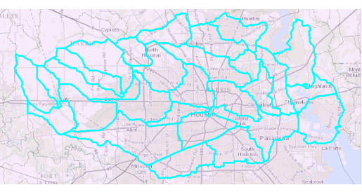
Part 3: Mapping Flowline Data
Next, you will add flowlines to your map, which were previously downloaded from NFIE.
- In the Table of Contents, check the Flowline and Catchment layers to make them visible.
Performing a spatial query
Now you would like to select out only the flowlines within the Buffalo-San Jacinto subbasin, but this is not possible with an attribute query, so you will instead use a spatial query.
...
- Export the selected Flowline features into your HydrologyLab geodatabase and name the new feature class “Flowlines”.
- Remove the original Flowline layer from the Table of Contents.
- Repeat step 1-7 using Catchment layer as Input Feature Layer and name the new feature class “Catchments”.
- Uncheck the Catchments layer, so it is no longer visible.
- In the Table of Contents, click the line symbol beneath the Flowlines layer name.
- In the ‘Symbology’ window under Gallery, select the Water (line) symbol and click OK.
- Open the Flowlines attribute table.
- Right-click the LENGTHKM field and select Statistics….
Symbolizing features using a single symbol
Calculating summary statistics for an attribute table field
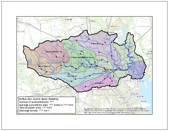
From the ‘Statistics of Flowlines’ window on the right of map display, you can see there are 543 flowlines in the Buffalo-San Jacinto basin whose average length is 1.94 km and total length is 1052 km.
...
4) What is the ratio of the total length of the streamlines to the total area of the Buffalo-San Jacinto catchments (called the drainage density) in km-1?
Symbolizing features by quantities using graduated symbols
- Open the Flowlines Symbology tab.
- Use Symbology drop down menu to select Graduated symbols.
- Use the ‘Field’ drop-down menu to select the Q0001C field, which contains the mean annual flow.
- Click the line next to Template to change the symbology of your flowlines.
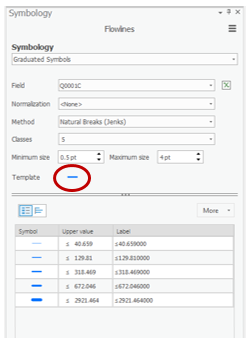
...
The flowlines should have graduated symbology based on their mean annual flow.
Part 4: Mapping Stream Gauge Data
Selecting data within subbasin
- In the table of contents, check the StreamGages layer which you brought in at the beginning with the Geographic feature dataset from the NFIEGeo_12 Geodatabase.
- On the Main menu, click Select By Location….
- For ‘Input Feature Layer’, check the StreamGage layer.
- For ‘Relationship’, use the drop-down menu to select within.
- For ‘Selecting Features’, use the drop-down menu to select Subbasin.
- Ensure your ‘Select by Location’ window appears as shown and click Run.

...
The stream gage site locations should be added to the map layout.
Part 5: Mapping Soils Data
Downloading SSURGO data
- In a web browser, go to http://arcgis.com.
...
Scroll down through the list of fields to see the wide variety of data available for each soil class. You may need to scroll to the right to see the actual values stored in these fields. In particular, you will be utilizing the data stored in the Available Water Storage 0-100 cm – Weighted Average field.
Geoprocessing: Clipping features
You will now clip the soil polygons to the extent of the Buffalo-San Jacinto subbasin.
...
- In the Table of Contents, right-click the Map Units layer and select Remove.
- Open the Soils Symbology tab.
- On the left, for ‘Show:’, click Quantities à Graduated colors.
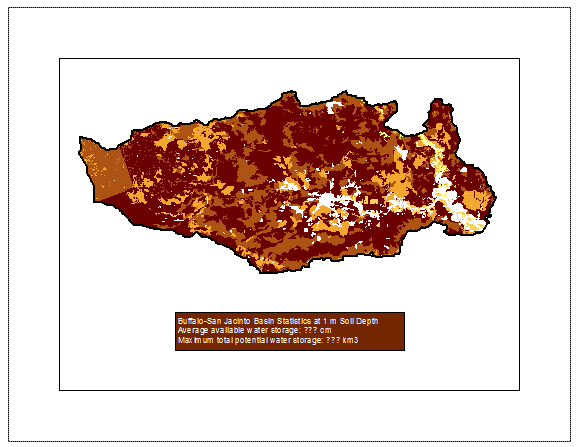
- Use the ‘Field’ drop-down menu to select the Available Water Storage 0-100 cm – Weighted Average field.
Symbolizing features by quantities using graduated colors
Notice that the density of the polygon outlines obscures the colors of the polygons themselves.
...
- What is the average available water storage (cm) in the Buffalo-San Jacinto subbasin?
- Based on your previous calculation of the area of the subbasin in km2, what volume of water (km3) could potentially be stored in the top 1 m of soil in the Buffalo-San Jacinto subbasin if the soil were fully saturated with water?
Exporting map documents
- To export both your Lab1Hydrology and Lab1Soils map documents, open each of them in turn and click the Project menu and select Export Map….
- Navigate to your HydrologyLab folder.
- Use the ‘Save as type:’ drop-down menu to select PDF.
- Click Save.
- Print both map PDFs to turn in
Deliverables
- Create an 8.5 x 11 layout with the following layers limited to the subbasin:
...