Page History

In this lab, you will practice downloading, manipulating, mapping, and analyzing publicly available hydrology data from a variety of online websites to study the Buffalo-San Jacinto watershed subbasin, which encompasses the greater Houston region. Specifically, you will work with watershed and flowline data from the National Flood Interoperability Experiment (NFIE), stream gage gauge data from the National Water Information System (NWIS), and soils data from the Soil Survey Geographic Database (SSURGO).

...

1. In the Insert tab, click ‘New Map’.
   

1. On Contents pane, click click Map name to rename it from Map to Lab1.
   

...

If you ever close the Catalog window, causing the Catalog tab to disappear, you can reopen it by clicking the Catalog View button on the Standard toolbar or by clicking , navigating to the Windows menu and selecting Catalog Pane.

The polygons in the Subwatershed layer represent all of the subwatersheds within the Texas-Gulf Coast Region 12, which you selected when initially downloading the data from the ArcGIS Online website. Now you will examine the attributes of this subwatershed data.

...

In the ‘Identify’ window, notice that the HUC_8 field contains the code 12040104, which corresponds to the Buffalo Bayou-San Jacinto subbasin. The first two digits (12) stand for the region (Texas-Gulf Region). The next two digits (1204) stand for the subregion (Galveston Bay-San Jacinto). The next two digits (120401) stand for the basin (San Jacinto). The last two digits (12040104) stand for the subbasin (Buffalo-San Jacinto). The additional two digits added to create the HUC-10 and HUC-12 codes stand for the watershed and subwatershed, respectively.

...

1. In the Geoprocessing pane, use ‘Layer Name or Table View’ drop-down menu to selectSubwatershed.
2. Use the ‘Selection Type’ drop-down menu to select New selection.
3. Click Add Clause.
   
   
   

1. SelectValues.

A list of all values stored in the HUC_8 field will appear in the box on the right.

1. Select SubwatershedHUC-8, and is equal to, in the first two fields.
2. Type ‘12040104’ in the last field.
3. Verify that your ‘Select By Attributes’ pane appears as shown on the following page and click Add.
   

...

Now you would like to highlight the boundary of the entire Buffalo-San Jacinto subbasin, but if you tried to change the outline of the current subwatersheds layer, it would change the outline around all subwatersheds. Instead, you will dissolve all the subwatersheds into a single subbasin feature stored in a new feature class inside your HydrologyLab geodatabase.

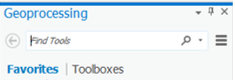
1. On Next to the Map tab, click the Analysis tab and select the Tools Tools.
2. On the search bar, type Dissolve and press Enter. Double-click Dissolve (Data Management Tools).
   

...

1. For ‘Input Features’, drag in the SubwatershedsNew layer from the Table of Contents or select the SubwatershedsNew option from the drop down box.
2. For ‘Output Feature Class’, rename the feature class from “SubwatershedsNew_Dissolve” to “Subbasin[g1] ”“Subbasin”.
3. For ‘Dissolve_Field(s)’, select the HUC_8 field, since this is the field containing the common subbasin value you wish to dissolve on.
4. Ensure your ‘Dissolve’ window appears as shown below, and click Run.
   

...

Now you would like to create a new layer based on the watersheds in the Buffalo-San Jacinto subbasin. In order to facilitate symbolization and labeling of the watershed names, you will now dissolve the subwatersheds into their respective watershed boundaries using the HUC-10 code.

1. Repeat steps 1-7 above, but for ‘Output Feature Class’, rename the feature class “Watersheds” and for ‘Dissolve_Field(s)’, check the HU_10_NAME field.

...

1. In the Table of Contents, right-click the Watersheds layer. Click Symbology.
2. Use the drop-down menu to select Unique values.
3. Use the ‘Value Field’ drop-down menu to select the HU_10_NAME field.
4. Use the ‘Color Ramp’ Scheme’ drop-down menu to select the color ramp of your choice.

...

Notice that the subwatersheds from the previous layer have now been grouped into 7 8 watersheds within the Buffalo-San Jacinto subbasin.

...

1. Export the selected Flowline features into your HydrologyLab geodatabase and name the new feature class “Flowlines”.
2. Remove the original Flowline layer from the Table of Contents.
3. Repeat step 1-7 using Catchment layer as Input Feature Layer and name the new feature class “Catchments”.
4. Uncheck the Catchments layer, so it is no longer visible.
5. In the Table of Contents, click the line symbol beneath the Flowlines layer name.
6. In the ‘Symbology’ window under Gallery, select the Water (line) symbol and click OK.
7. Open the Flowlines attribute table.
8. Right-click the LENGTHKM field and select Statistics….

...

1. In the search bar in the top right corner, type Houston, TX.
   

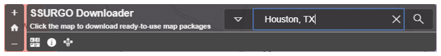
1. Click in the Buffalo-San Jacinto subbasin to select it and click the Download link.
   

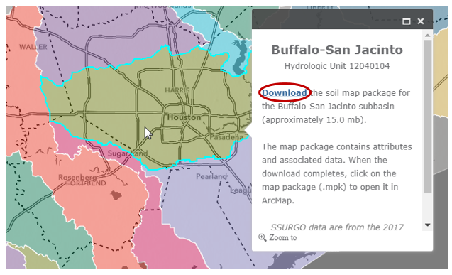
1. Right-click on your downloaded BuffaloSanJacinto_12040104.mpk ppkx file and select Show in folder. Copy its the file path location.
2. Open ArcGIS Pro, click Insert tab and select Import Map.
   Image Removed
3. Paste the file path location to import window. Press Enter. Select BuffaloSanJacinto_12040104.mpk file.
4. Click OK.
   Image Removed
5. .
6. Navigate back to your HydrologyLab folder.
7. Paste the BuffaloSanJacinto_12040104.ppkx file directly inside your HydrologyLab folder. Do NOT paste it inside the Hydrologylab.gdb geodatabase.
8. Single click the file and press Enter.
9. A new ArcGIS Pro window will open. You will complete Part 5 using this window. Do not delete your previous ArcGIS Pro window. 

A map package (.mpk), contains both a map document (.mxd) and all data layers referenced by that map document. A The new instance of ArcMap ArcGIS Pro will open showing the different soil classes within the subbasin.

...

1. In the Table of Contents, right-click the Map Units layer and select Remove.
2. Open the Soils Symbology tabpane.
3. On the left, for ‘Show:’, click Quantities à Click Graduated colors.
4. Use the ‘Field’ drop-down menu to select the Available Water Storage 0-100 cm – Weighted Average field.

...

1. To export both your Lab1Hydrology and Lab1Soils map documents, open each of them in turn and click the Project Share menu and select Export Map…Layout….
2. Navigate to your HydrologyLab folder.
3. Use the ‘Save as type:’ drop-down menu to select PDF.
4. Click Save Export.
5. Print both map PDFs to turn in

...