| Info |
|---|
This guide was created by the staff of the GIS/Data Center at Rice University and is to be used for individual educational purposes only. The steps outlined in this guide require access to ArcGIS Pro software and data that is available both online and at Fondren Library. |
Table of Contents
| Info |
|---|
The following text styles are used throughout the guide: Explanatory text appears in a regular font.
Folder and file names are in italics. Names of Programs, Windows, Panes, Views, or Buttons are Capitalized. 'Names of windows or entry fields are in single quotation marks.' "Text to be typed appears in double quotation marks." |
| Info |
|---|
The following step-by-step instructions and screenshots are based on the Windows 10 operating system with the Windows Classic desktop theme and ArcGIS Pro 3.2.0 software. If your personal system configuration varies, you may experience minor differences from the instructions and screenshots. |
In this lab, you will practice downloading, manipulating, mapping, and analyzing publicly available hydrology data from a variety of online websites to study the Buffalo-San Jacinto watershed subbasin, which encompasses the greater Houston region. Specifically, you will work with watershed and flowline data from the National Flood Interoperability Experiment (NFIE), stream gauge data from the National Water Information System (NWIS), and soils data from the Soil Survey Geographic Database (SSURGO).
Part 1: Creating a New GIS Project
In this lab, you will practice downloading, manipulating, mapping, and analyzing publicly available hydrology data from a variety of online websites to study the Buffalo-San Jacinto watershed subbasin, which encompasses the greater Houston region. Specifically, you will work with watershed and flowline data from the National Flood Interoperability Experiment (NFIE), stream gauge data from the National Water Information System (NWIS), and soils data from the Soil Survey Geographic Database (SSURGO).
Part 1: Setting Up a GIS Project
Creating a new project folder
First, you will need to establish a project folder, where you will store all of the files associated with this lab assignment. When working in a public computer lab environment, we recommend saving your work on an external USB drive. For the purposes of illustration throughout these lab instructions, the project folder will be located directly on a USB drive, which is mapped as the F: drive, though your USB drive letter may vary. If you wish to nest your project folder inside other folders within the file organization scheme on your USB drive, ensure that no spaces or special characters are used anywhere along the entire file path of your project folder.
- Using Windows Explorer, navigate to the location where you would like to locate your project folder (likely the E: or F: drive).
- Create a new folder inside your selected location and name it “HydrologyLab”. Remember not to use any spaces. Note the full file path of your HydrologyLab folder.
Connecting to a project folder
Now that you have created a project folder for this lab, you will need to create a new ArcGIS Pro project in it.
- On the Desktop,
On the Desktop,
click the Start menu and select ArcGIS > ArcGIS Pro.
- If the 'ArcGIS Sign In' window appears, sign in using your Rice organizational account. (Detailed Instructions)
- In the ‘ArcGIS Pro’ window, under the 'New' section, select the Map template.

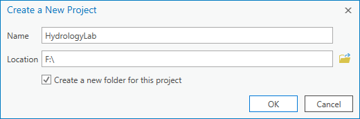
- In the ‘Create a New Project’ window, for 'Name', type " HydrologyLab ".
- For 'Location', click the Browse button to navigate to the HydrologyLab folder created. Once the HydrologyLab folder is selected, click OK.
- Uncheck Create a new folder for this project. Click OK.
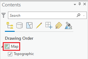
Because you created a new project using the Map template, the project opens with a single map already created; however, it is generically named Map, so you will give it a more descriptive name to differentiate it from the maps created in future labs.
...
Part 2: Mapping Watershed Data
Downloading NFIE data
Your project folder and geodatabase have been created, so you are ready to download your first set of online GIS data. You will start by downloading data from the National Flood Interoperability Experiment (NFIE), which is searchable on the ArcGIS Online platform.
- In a web browser, go towww.arcgis.com.
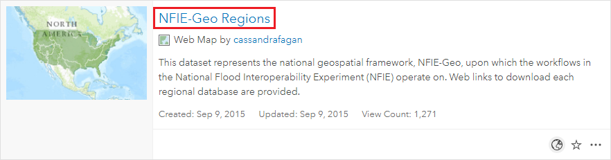
- In the search box in the top right of the website, type “NFIE-Geo Regions”.
If no items are returned, it is likely because you are signed in to your Rice account and the content is limited to Rice University content by default.
...
Adding feature data in ArcMap
Unfortunately, any changes you make to files outside of ArcGIS Pro are not automatically reflected inside ArcGIS Pro. Since you just added new files to your HydrologyLab folder, you will need to refresh your HydrologyLab folder in order for them to appear.
- In the Catalog pane on the right of the map view, expand Folders, right-click your HydrologyLab folder, and select Refresh.
- Expand the HydrologyLab folder > NFIEGeo_12.gdb geodatabase > Geographic feature dataset to preview what feature classes, or layers, it contains.
Drag the Geographic feature dataset from the Catalog pane into the Lab1 map view.
If you ever close the Catalog pane, you can reopen it by clicking the View tab on the ribbon and then clicking the Catalog Pane button.
The polygons in the Subwatershed layer represent all of the subwatersheds within the Texas-Gulf Coast Region 12, which you selected when initially downloading the data from the ArcGIS Online website. Now you will examine the attributes of this subwatershed data.
- In the Table of Contents, right-click the Subwatershed layer and select Attribute Table. Expand the size of the table, if desired.
You will notice three of the columns are labeled HUC_8, HUC_10, and HUC_12, which correspond to the subbasin, watershed, and subwatershed codes respectively. HUC stands for hydrologic unit code, which is a unique identification number assigned to each hydrologic unit in the United States. Further to the right, you will see additional columns containing the actual names of the HUC-10 watersheds and HUC-12 subwatersheds.
- Close the Subwatershed attribute table.
Adding an online basemap
First, you would like to identify the subwatersheds within the greater Houston region, but, without any additional reference layers regarding streets or administrative boundaries, this would be very difficult to do. Fortunately, you can utilize various basemaps of the world hosted online by Esri, rather than having to obtain all of the GIS reference layers yourself. Because these basemaps are being hosted online, they cannot be edited and can sometimes be slow to load.
Though the Topographic basemap has already been added to your map by default, it appears in the background and is visually obscured by the other data layers.
- In the Table of Contents, uncheck the StreamGage, Flowline, Catchment and Waterbody layers, leaving only the Subwatershed layer visible.
The basemap is still not visible beneath the Subwatersheds layer, so you will need to make that layer transparent.
...
Now the basemap should be visible beneath the subwatersheds.
Identifying features
Ultimately, you want to select all of the subwatersheds that lie within the Buffalo-San Jacinto subbasin in which Houston is located, but first you will need to look up the HUC-8 code corresponding to this subbasin.
- On the ribbon, click the Map tab and ensure that the Explore tool is selected.
- Use the navigation tools to zoom in to the Houston region.
- In the map view, click near the center of Houston.
In the ‘Pop-up’ window, notice that the HUC_8 field contains the code 12040104, which corresponds to the Buffalo Bayou-San Jacinto subbasin. The first two digits (12) stand for the region (Texas-Gulf Region). The next two digits (1204) stand for the subregion (Galveston Bay-San Jacinto). The next two digits (120401) stand for the basin (San Jacinto). The last two digits (12040104) stand for the subbasin (Buffalo-San Jacinto). The additional two digits added to create the HUC-10 and HUC-12 codes stand for the watershed and subwatershed, respectively.
- Close the 'Pop-up' window.
Performing an attribute query
Now you are ready to perform an attribute query to select all of the subwatersheds within the Buffalo-San Jacinto subbasin (HUC-8 = 12040104).
...
- .
Navigate to the location in which you would like to store your HydrologyLab project folder and click OK.
Info A project folder is where you will store all of the files associated with this lab assignment. When working in a public computer lab environment, we recommend saving your work on an external USB drive. If you wish to nest your project folder inside other folders on your USB drive, or if you are using the hard drive on personal computer, ensure that no spaces or special characters are used anywhere along the entire file path of your project folder. The default project location on your personal computer is C:\Users\[ username ]\Documents\ArcGIS\Projects.
In order to connect to a folder, you often have to be able to select the folder from the file browser on the right, rather than in the Navigation pane on the left. For example, if you wanted to store the project on an external USB F:\ drive, you would need to single-click Computer in the Navigation pane on the left and then single-click F:\ in the file browser on the right.
- Once the HydrologyLab folder is selected, click OK.
- Ensure Create a new folder for this project is checked.
- Click OK.
Because you created a new project using the Map template, the project opens with a single map already created; however, it is generically named Map, so you will give it a more descriptive name to differentiate it from the maps created in future labs.
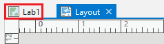
- In the Contents pane, click Map once to select it. Then, click directly on the Map text a second time and rename it " Lab1Hydrology ".
Part 2: Mapping Watershed Data
Downloading NFIE data
Your project folder and geodatabase have been created, so you are ready to download your first set of online GIS data. You will start by downloading data from the National Flood Interoperability Experiment (NFIE), which is searchable on the ArcGIS Online platform.
- In a web browser, go to www.arcgis.com .
- In the search box in the top right of the website, type “NFIE-Geo Regions”.
If no items are returned, it is likely because you are signed in to your Rice account and the content is limited to Rice University content by default.
- If necessary, in the 'Filters' section on the left sidebar, toggle off Only search in Rice University, at which point the proper layer should appear.

- Click the NFIE-Geo Regions web map.
- On the right, click to Open in Map Viewer.
- On the map, click to select the Texas-Gulf region, which encompasses Houston.
- In the table in the pop-up, next to Hydroshare, click View.
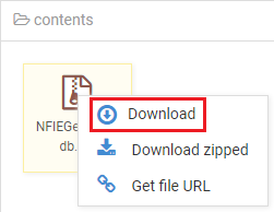
- In the Content section, right-click the NFIEGeo_12.gdb.zip file and select Download.
- Navigate to the location where the zipped file has been downloaded.
- Right-click the downloaded NFIEGeo_12.gdb zip file and select Extract All….
- In the ‘Extract Compressed (Zipped) Folders' window, click Extract.
- In the new extracted folder window that opens, right-click the extracted NFIEGeo_12.gdb folder and select and Copy.
- Navigate back to your HydrologyLab folder.
- Paste the NFIEGeo_12.gdb folder directly inside your HydrologyLab folder. Do NOT paste them inside the HydrologyLab.gdb geodatabase.
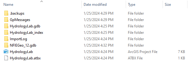
- Ensure that your HydrologyLab folder appears as shown below.
- Return to ArcGIS Pro.
Adding feature data in ArcGIS Pro
Unfortunately, any changes you make to files outside of ArcGIS Pro are not automatically reflected inside ArcGIS Pro. Since you just added new files to your HydrologyLab folder, you may need to refresh your HydrologyLab folder in order for them to appear.
- In the Catalog pane on the right of the map view, expand Folders, right-click your HydrologyLab folder, and select Refresh.
- Expand the HydrologyLab folder > NFIEGeo_12.gdb geodatabase > Geographic feature dataset to preview what feature classes, or layers, it contains.
Drag the Geographic feature dataset from the Catalog pane into the Lab1Hydrology map view.
If you ever close the Catalog pane, you can reopen it by clicking the View tab on the ribbon and then clicking the Catalog Pane button.
The polygons in the Subwatershed layer represent all of the subwatersheds within the Texas-Gulf Coast Region 12, which you selected when initially downloading the data from the ArcGIS Online website. Now you will examine the attributes of this subwatershed data.
- In the Contents pane, right-click the Subwatershed layer and select Attribute Table. Expand the size of the table, if desired.
You will notice three of the columns are labeled HUC_8, HUC_10, and HUC_12, which correspond to the subbasin, watershed, and subwatershed codes respectively. HUC stands for hydrologic unit code, which is a unique identification number assigned to each hydrologic unit in the United States. Further to the right, you will see additional columns containing the actual names of the HUC-10 watersheds and HUC-12 subwatersheds.
- Close the Subwatershed attribute table.
Adding an online basemap
First, you would like to identify the subwatersheds within the greater Houston region, but, without any additional reference layers regarding streets or administrative boundaries, this would be very difficult to do. Fortunately, you can utilize various basemaps of the world hosted online by Esri, rather than having to obtain all of the GIS reference layers yourself. Because these basemaps are being hosted online, they cannot be edited and can sometimes be slow to load.
Though the Topographic basemap has already been added to your map by default, it appears in the background and is visually obscured by the other data layers.
- In the Contents pane, uncheck the StreamGage, Flowline, Catchment and Waterbody layers, leaving only the Subwatershed layer visible.
The basemap is still not visible beneath the Subwatersheds layer, so you will need to make that layer transparent.
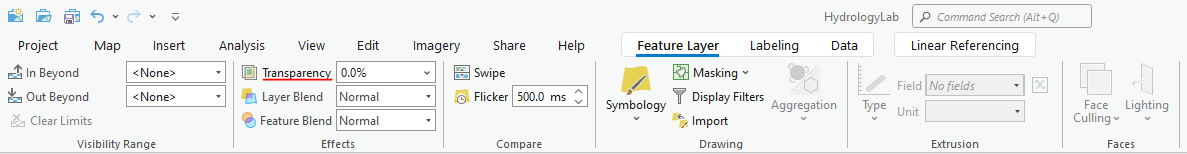
- In the Contents pane, click the Subwatershed layer to select it.
- On the ribbon, click the Feature Layer tab.
- In the Effects group, type “60” to change the transparency of the layer.
Now the basemap should be visible beneath the subwatersheds.
Identifying features
Ultimately, you want to select all of the subwatersheds that lie within the Buffalo-San Jacinto subbasin in which Houston is located, but first you will need to look up the HUC-8 code corresponding to this subbasin.
- On the ribbon, click the Map tab and ensure that the Explore tool is selected.
- Use the navigation tools to zoom in to the Houston region.
- In the map view, click near the center of Houston.
In the ‘Pop-up’ window, notice that the HUC_8 field contains the code 12040104, which corresponds to the Buffalo Bayou-San Jacinto subbasin. The first two digits (12) stand for the region (Texas-Gulf Region). The next two digits (1204) stand for the subregion (Galveston Bay-San Jacinto). The next two digits (120401) stand for the basin (San Jacinto). The last two digits (12040104) stand for the subbasin (Buffalo-San Jacinto). The additional two digits added to create the HUC-10 and HUC-12 codes stand for the watershed and subwatershed, respectively.
- Close the 'Pop-up' window.
Performing an attribute query
Now you are ready to perform an attribute query to select all of the subwatersheds within the Buffalo-San Jacinto subbasin (HUC-8 = 12040104).
- On the Map tab, click the Select by Attributes button.

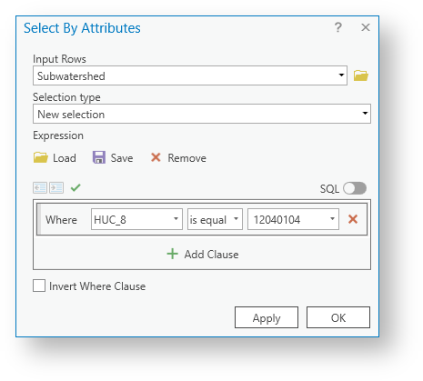
- In the 'Select By Attributes' window, use the ‘Input Rows’ drop-down menu to select the Subwatershed layer, if necessary.
- Use the ‘Selection Type’ drop-down menu to select New selection.
- Click New expression.
- For the first two fields, select HUC-8 , and is equal to .
- Type "12040104" in the last field.
- Verify that your ‘Select By Attributes’ window appears as shown below and click OK.
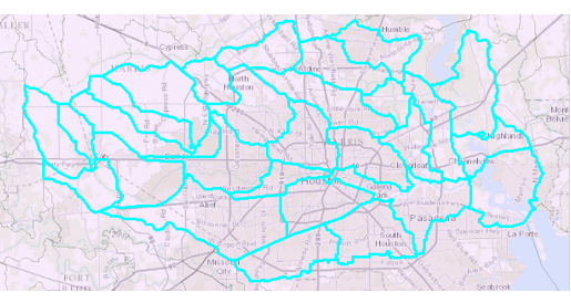
- In the Contents pane, right-click the Subwatershed layer and select Selection > Zoom To Selection.
Exporting selected features
Now that the Buffalo-San Jacinto subwatersheds have been selected, they can be exported into a separate layer stored in your HydrologyLab geodatabase.
- In the Contents pane, right-click the Subwatershed layer and select Data > Export Features.
By default, the ‘Export Features’ window will only export the selected features using the coordinate system of the data source. Also notice that the output location defaults to the HydrologyLab geodatabase, because that is your default geodatabase for this project.
- For ‘Output Name’, type “ SubwatershedsNew ”.
- Ensure your ‘Export Features’ window appears as shown below and click OK.

Since you’ve exported the particular subwatersheds of interest, you may now remove the master Subwatersheds layer from your map.
- In the Contents pane, right-click the Subwatershed layer and select Remove.
Saving ArcGIS projects
At this point, it is a good idea to save your map document and to continue saving regularly.
- On the Quick Access toolbar, click the Save button.
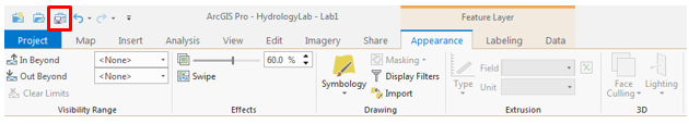
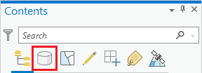
At the top of the Contents pane window, notice that the leftmost List By Drawing Order button is currently selected.
- At the top of the Contents pane, click the List By Source button.
The Data Source tab displays the full file path locations of all the data layers referenced in your map. Notice that the majority of layers are still stored in the originally downloaded NFIEGeo_12 geodatabase, but the SubwatershedsNew layer you just exported is now stored in your HydrologyLab project geodatabase.
- At the top of the Contents pane, click the List By Drawing Order button to return to the list of data layers.

Geoprocessing: Dissolving features
Now you would like to highlight the boundary of the entire Buffalo-San Jacinto subbasin, but, if you tried to change the outline of the current Subwatersheds layer, it would change the outline around all subwatersheds. Instead, you will dissolve all the subwatersheds into a single subbasin feature stored in a new feature class inside your HydrologyLab geodatabase.
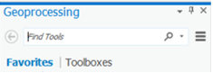
- On the ribbon, click the Analysis tab and click the Tools button, which will open the Geoprocessing pane on the right.
Notice that at the bottom of the Geoprocessing pane, you now see the Catalog and Geoprocessing tabs. Any future panes that are opened will create additional tabs at the bottom.
- At the top of the Geoprocessing pane, in the 'Find Tools' box, type "dissolve" and press Enter.
- Click Dissolve (Data Management Tools).
- In the top right corner of the ‘Dissolve’ tool pane, hover over the question mark icon.
Read the ‘Dissolve’ window help and review the sample illustration. Notice that this tool dissolves boundaries based on common values in a particular field. In this case, you will dissolve the subwatersheds based on their common subbasin value, resulting in a file showing only the larger subbasin boundary. If you were to click on the question mark icon, it would open up the full Dissolve tool documentation on the ArcGIS Pro help website.
- For ‘Input Features’, drag in the SubwatershedsNew layer from the Contents pane or select the SubwatershedsNew option from the drop down box.
- For ‘Output Feature Class’, rename the feature class from “SubwatershedsNew_Dissolve” to “ Subbasin ”.
- For ‘Dissolve_Field(s)’, select the HUC_8 field, since this is the field containing the common subbasin value you wish to dissolve on.
- Ensure your ‘Dissolve’ tool appears as shown below, and click Run.

- In the Contents pane, toggle the new Subbasin layer off and on to get a better idea of the result of the Dissolve tool.
- In the Contents pane, right-click the Subbasin layer and select Attribute Table.
Notice that only the dissolve field, in this case the HUC_8 field, was preserved. Because multiple subwatersheds were dissolved into a single subbasin, it is not possible to retain all of the attributes of each separate subwatershed.
- Close the Subbasin attribute table.
In order to see all the layers simultaneously, you will give the subbasin boundary a hollow outline.
- In the Contents pane, click the rectangle symbol beneath the Subbasin layer name to open the Symbology pane on the right.
- Near the top of the Symbology pane, click the Properties tab.

- For ‘Color:’, use the drop-down menu to select No Color.
- For ‘Outline Color:’, used the drop-down menu to select Black.
- For ‘Outline Width:’, type “2”.
- Click Apply.
Now you would like to create a new layer based on the watersheds in the Buffalo-San Jacinto subbasin. In order to facilitate symbolization and labeling of the watershed names, you will now dissolve the subwatersheds into their respective watershed boundaries using the HUC-10 code.
- At the bottom of the Symbology pane, click the Geoprocessing tab.
- For ‘Input Features’, leave the SubwatershedsNew layer previously entered.
- For ‘Output Feature Class’, rename the feature class from Subbasin to “ Watersheds ”.
- For ‘Dissolve_Field(s)’, select the HUC_10_NAME field.
- Click Run.
While you could have also dissolved using the HU_10 field, the watershed name is probably more meaningful to you than the HU_10 code. You no longer need the SubwatershedsNew layer for this section. The rest of the analysis will be done with the new Watersheds layer.
- In the Contents pane, uncheck the original SubwatershedsNew layer.
- In the Contents pane, drag the Subbasin layer above the Watersheds layer, so it is fully visible again.
Symbolizing features by categories using unique values
Now that you have generated the watershed features within the Buffalo-San Jacinto subbasin, you will symbolize them based on their HUC-10 watershed name.
- In the Contents pane, right-click the Watersheds layer and select Symbology.
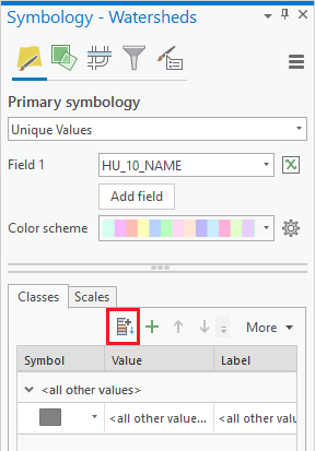
- In the Symbology pane, use the 'Primary symbology' drop-down menu to select Unique Values.
- Use the ‘Field 1’ drop-down menu to select the HU_10_NAME field.
- Use the ‘Color Scheme’ drop-down menu to select the color ramp of your choice.

- On the bottom half of the Symbology pane, if only one category called <all other values> is listed, as shown below, click the Add all values button.
Notice that the subwatersheds from the previous layer have now been grouped into 8 watersheds within the Buffalo-San Jacinto subbasin. Notice also that the transparency originally applied to the Subwatershed layer, was maintained as the layer was re-exported and then merged, such that the Topographic basemap still appears through it.
- Ensure that the Watersheds layer is selected in Contents pane.
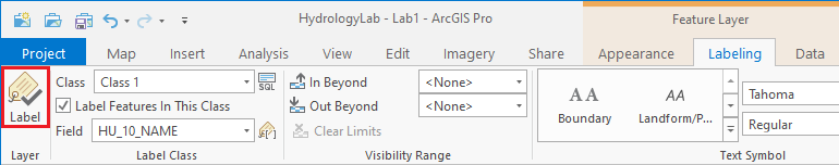
- On the ribbon, click the Feature Layer contextual Labeling tab.
- In the Label Class group, for 'Field', ensure the HU_10_NAME field is selected.
- In the Layer group, click the Enable Labeling button to turn on the labels.
Creating a layout
- On the ribbon, click the Insert tab.
- In the Project group, click the New Layout button and, under the 'ANSI - Landscape' section, click Letter 8.5" x 11".
- On the ribbon, click the Map Frame group and, under the 'Lab1Hydrology' map section, select the second frame that is labeled with the scale, such as 1:600,000.

- Under the 'Rice Bus Routes' map section, select the second frame that is labeled with a scale, such as 1:600:000.
- Click and hold near the top left corner of the layout page and drag the rectangle near the bottom right corner or the layout page.
- In the Contents pane, right-click the Watersheds layer and select Zoom to Layer.
Using techniques you learned last week, create a suitable map, as described for the map layout to be turned in below. All map elements, such as text, legends, north arrows, and scale bars can be added to the layout from the Insert tab on the ribbon.
- Save your project
FOR MAP LAYOUT TO BE TURNED IN
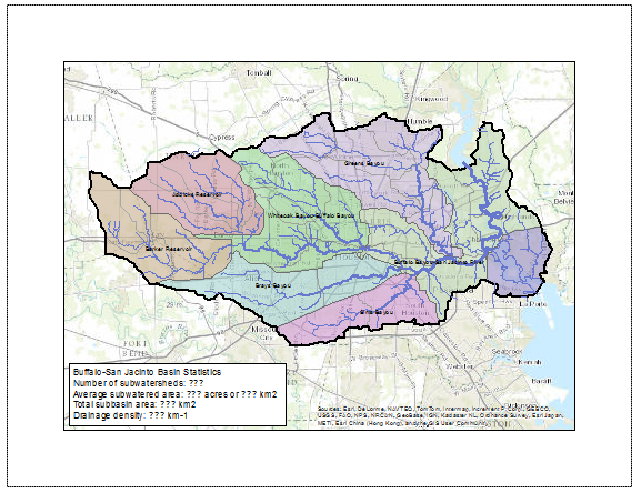
Create an 8.5" x 11" layout clearly delineating the subbasin and watersheds on top of a basemap, with the symbology and labels corresponding to the watersheds. You may need to further adjust the order of your layers in the Contents pane and their symbology.

Part 3: Mapping Flowline Data
Next, you will add flowlines to your map, which were previously downloaded from NFIE.
- At the top left of your Layout view, click the Lab1Hydrology map tab to return to your map view.
- In the Contents pane, check the Flowline and Catchment layers to make them visible.
Performing a spatial query
Now you would like to select only the flowlines and catchments within the Buffalo-San Jacinto subbasin, but this is not possible with an attribute query, so you will instead use a spatial query.
- On the ribbon, click the Map tab.
- In the Selection group, click the Select By Location button.
- For ‘Input Features’, use the drop-down menu to select the Flowline layer.
- Use the second 'Input Features' drop-down menu to select the Catchment layer.
- For ‘Relationship’, use the drop-down menu to select Have their center in. (This setting ensures that catchments and flowlines which share the outside border with the subbasin will not also get selected.)
- For ‘Selecting Features’, use the drop-down menu to select the Subbasin layer.
- Ensure your ‘Select by Location’ window appears as shown below and click OK.

All of the flowlines and catchment areas that are within the subbasin are now selected.
- Export the selected Flowline features into your HydrologyLab geodatabase and name the new feature class “ Flowlines ”.
- Remove the original Flowline layer from the Contents pane.
- Export the selected Catchment features into your HydrologyLab geodatabase and name the new feature class “ Catchments ”.
- Remove the original Catchment layer from the Contents pane.
- Uncheck the new Catchments layer, so it is no longer visible.
Symbolizing features using a single symbol
- In the Contents pane, click the line symbol beneath the Flowlines layer name.
- At the top of the Symbology pane, click the Gallery tab and select the Water (line) symbol.
Calculating summary statistics for an attribute table field
- Open the Flowline s attribute table.
- Scroll right to the 8th field and right-click the LENGTHKM field name and select Statistics.
From the Chart Properties pane on the right, you can see there are 543 flowlines in the Buffalo-San Jacinto basin whose average length is 1.94 km and total length is 1052 km.
- View the statistics for the AreaSqKM field in the Catchments attribute table.
Based on the statistics you have just seen, calculate the answers to the questions listed for the map layout to be turned in below. In order to add the statistics to your map layout, you will insert a rectangle text element.
- At the top left of your map view, click the Layout tab to return to your layout view.
- On the ribbon, click the Insert tab.
- In the Graphics and Text group, click the Rectangle text button.

- Drag a rectangle on your map layout to insert a rectangle text element.
You can edit the text and customize the rectangle appearance by double-clicking on the rectangle text element and using the 'Format Text' Element pane on the right.
- Save your project.
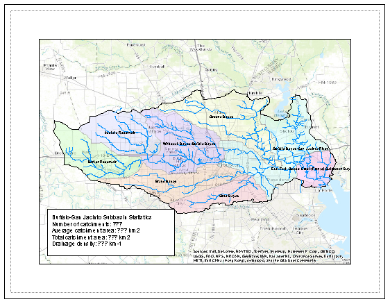
FOR MAP LAYOUT TO BE TURNED IN
Add a text box to the layout containing the answers to the following questions:
- How many catchments are there in the Buffalo-San Jacinto subbasin?
- What is their average area in acres and in km2? (Look up conversion factor.)
- What is the total area of catchments in km2?
- What is the ratio of the total length of the streamlines to the total area of the Buffalo-San Jacinto catchments (called the drainage density) in km-1?
Symbolizing features by quantities using graduated symbols
- Return to the Lab1Hydrology map view.
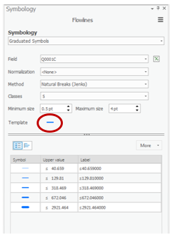
- Open the Flowlines Symbology tab.
- Use 'Primary Symbol' drop down menu to select Graduated symbols.
- Use the ‘Field’ drop-down menu to select the Q0001C field, which contains the mean annual flow.
- Click the line next to Template to change the symbology of your flowlines.
- Save your project.
FOR MAP LAYOUT TO BE TURNED IN
The flowlines should have graduated symbology based on their mean annual flow.
Part 4: Mapping Stream Gauge Data
Selecting data within subbasin
- In the Contents pane, check the StreamGage layer which you brought in at the beginning with the Geographic feature dataset from the NFIEGeo_12 Geodatabase.
- On the ribbon, click the Map tab.
- Click the Select By Location button.
- For ‘Input Features’, use the drop-down menu to select the StreamGage layer.
- For ‘Relationship’, use the drop-down menu to select Within.
- For ‘Selecting Features’, use the drop-down menu to select the Subbasin layer.
- Click OK.
All of the stream gages that are within the subbasin are now selected.
- Export the selected StreamGage features into your HydrologyLab geodatabase and name the new feature class “ SubbasinStreamGages ”.
- Remove the original StreamGage layer from the Contents pane.
Export a layout
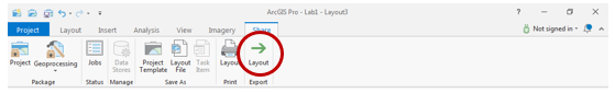
- Return to the Layout view.
- On the ribbon, click the Share tab and click the Layout button in the Export group to open the Export Layout pane on the right.
- In the Export Layout pane, use the 'File Type' drop-down menu to select PDF.
- For 'Name', type "Lab 1 Hydrology" and click Export.
- Save your project.
FOR MAP LAYOUT TO BE TURNED IN
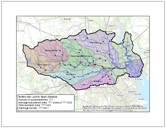
The stream gage site locations should be added to the map layout.
Part 5: Mapping Soils Data
Downloading SSURGO data
- In a web browser, go to http://arcgis.com.
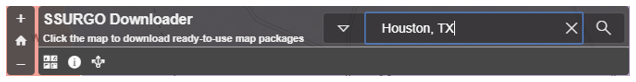
- On the top right search bar, search for "SSURGO Downloader".
- Again, if necessary, in the 'Filters' section on the left sidebar, toggle off Only search in Rice University, at which point the proper layer should appear.

- Click the SSURGO Downloader web mapping application.

- On the right side of the webpage click the View Application button.

- In the search bar in the top corner, type "Houston, TX".
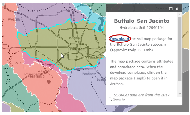
- Click in the Buffalo-San Jacinto subbasin to select it and click the Download link.
- Right-click on your downloaded BuffaloSanJacinto_12040104.ppkx file and select Show in folder. Copy the file.
- Navigate back to your HydrologyLab folder.
- Paste the BuffaloSanJacinto_12040104.ppkx file directly inside your HydrologyLab folder. Do NOT paste it inside the Hydrologylab.gdb geodatabase.
- Single-click the .ppkx file to select it and press Enter.
A new ArcGIS Pro application window will open. You will complete Part 5 using this window, but do not close your previous ArcGIS Pro window.
A packaged project file (.ppkx), contains both a project (.aprx) and all data layers referenced in the project in a project geodatabase (.gdb). The new instance of ArcGIS Pro will open showing the different soil classes within the subbasin.
- In the Contents pane, right-click the Subbasin layer and select Zoom To Layer.
- On the Map tab, click the Explore button.
- In the Contents pane, uncheck the Subbasin layer, so that it will not be queried in the next step.
- In the Map view, click on any of the soil classes.
Scroll down through the list of fields to see the wide variety of data available for each soil class. You may need to scroll to the right to see the actual values stored in these fields. In particular, you will be utilizing the data stored in the Available Water Storage 0-100 cm – Weighted Average field.
Geoprocessing: Clipping features
You will now clip the soil polygons to the extent of the Buffalo-San Jacinto subbasin.
- On the ribbon, click the Analysis tab and click the Tools button.
- At the top of the Geoprocessing pane, in the 'Find Tools' search bar, type "clip" and press Enter.
- Click Clip (Analysis Tools).
Read the ‘Clip’ window help and review the sample illustration. Notice that this tool clips one dataset to the extent, or shape, of another dataset.
- For ‘Input Features’, use the drop-down menu to select the Mapunits layer.
- For ‘Clip Features’, use the drop-down menu to select the Subbasin layer.
Hover over the ‘Output Feature Class’ field and note that the file path did not default to your HydrologyLab geodatabase, but instead to the default geodatabase that was referenced in the map package you downloaded. You will change this to your default project geodatabase.
- For 'Output Feature Class', click the Browse button.
- Navigate to your HydrologyLab folder and double-click the HydrologyLab geodatabase.
- For 'Name', type “ Soils ” and click Save.
- In the Geoprocessing pane, again hover over the ‘Output Feature Class’ field to ensure the output Soils feature class will be stored in your HydrologyLab geodatabase and click Run.
Notice that the resulting Soils layer maintains the soil class boundaries, but limits the extent of the soils layer to the extent of the subbasin boundary.
You will now return to your main HydrologyLab project application window.
- Close the BuffaloSanJacinto_12040104 project in ArcGIS Pro without saving.
- Return to your HydrologyLab project.
- On the ribbon, click the Insert tab.
- On the far left, click the New Map button.
- In the Contents pane, click Map once to select it. Then, click directly on the Map text a second time and rename it " Lab1Soils ".
- At the bottom of the far right pane, click the Catalog tab.
- Right-click the HydrologyLab.gdb geodatabase and select Refresh.
- Drag the newly clipped Soils feature class from the Catalog pane to the Lab1Soils map view.
- Also, drag the Subbasin feature class from the Catalog pane to the Lab1Soils map view.
- Symbolize the Subbasin layer using the same symbology as you used in the Lab1Hydrology map, with no color and a black outline.
Symbolizing features by quantities using graduated colors
- In the Contents pane, click the Soils layer to select it.
- If necessary, open the Symbology pane.
- For 'Primary symbology', select Graduated Colors.
- For ‘Field’,
...
Exporting selected features
Now that the Buffalo-San Jacinto subwatersheds have been selected, they can be exported into a separate layer stored in your HydrologyLab geodatabase.
- In the Table of Contents, right-click the Subwatershed layer and select Data > Export Features….
Notice that, by default, the ‘Export Data’ window is set to export only the selected features using the coordinate system of the data source. Also notice that the output feature class defaults to the HydrologyLab geodatabase, because you initially set this as your default geodatabase.
...
Since you’ve exported the particular subwatersheds of interest, you may now remove the master Subwatersheds layer from your map document.
- Right-click the Subwatershed layer and select Remove.
Saving ArcGIS projects
At this point, it is a good idea to save your map document and to continue saving regularly.
- On the Quick Access toolbar, click the Save button.
At the top of the Table of Contents window, notice that the leftmost List By Drawing Order button is currently selected.
- At the top of the Table of Contents, click the List By Source button.

The Source tab displays the full file path locations of all the data layers referenced in your map document. By default, the map document will store this full file path to all of your data files.
- At the top of the Table of Contents, click the List By Drawing Order button to return to the list of data layers.
Geoprocessing: Dissolving features
Now you would like to highlight the boundary of the entire Buffalo-San Jacinto subbasin, but if you tried to change the outline of the current subwatersheds layer, it would change the outline around all subwatersheds. Instead, you will dissolve all the subwatersheds into a single subbasin feature stored in a new feature class inside your HydrologyLab geodatabase.
...
Read the ‘Dissolve’ window help and review the sample illustration. Notice that this tool dissolves boundaries based on common values in a particular field. In this case, you will dissolve the subwatersheds based on their common subbasin value, resulting in a file showing only the larger subbasin boundary.
...
Notice that only the dissolve field, in this case the HUC_8 field, was preserved. Because multiple subwatersheds were dissolved into a single subbasin, it is not possible to retain all of the attributes of each separate subwatershed.
- Close the attribute table.
In order to see all the layers simultaneously, you will give the subbasin boundary a hollow outline.
- In the Table of Contents, click the rectangle symbol beneath the Subbasin layer name to open the ‘Symbology’ tab.
- On the top of the tab, click Properties.
- For ‘Color:’, use the drop-down menu to select No Color.
- For ‘Outline Color:’, used the drop-down menu to select Black.
- For ‘Outline Width:’, type “2”.
- Click Apply.
Now you would like to create a new layer based on the watersheds in the Buffalo-San Jacinto subbasin. In order to facilitate symbolization and labeling of the watershed names, you will now dissolve the subwatersheds into their respective watershed boundaries using the HUC-10 code.
- Repeat steps above, but for ‘Output Feature Class’, rename the feature class “Watersheds” and for ‘Dissolve_Field(s)’, check the HU_10_NAME field.
You no longer need the original subwatersheds layer for this section. The rest of the analysis will be done with the new Watersheds layer.
- In the Table of Contents, uncheck the original SubwatershedsNew layer.
- In the Table of Contents, drag the Subbasin layer above the Watersheds layer, so it is fully visible again.
Symbolizing features by categories using unique values
Now that you have generated the watershed features within the Buffalo-San Jacinto subbasin, you will symbolize them based on their HUC-10 watershed name.
...
While you could have also dissolved using the HU_10 field, the watershed name is probably more meaningful to you than the HU_10 code.
Notice that the subwatersheds from the previous layer have now been grouped into 8 watersheds within the Buffalo-San Jacinto subbasin.
...
Depending on your screen size, you may notice the easternmost watershed does not get labeled if there is not adequate space for the required text. This could be adjusted using advanced labeling techniques, but you will leave the map as is.
Creating a layout
- On the main tab, click Insert > New Layout > ANSI Landscape > Letter.
- Click Insert tab and click Map Frame.
- Select the Lab1 map under Map.

- Select Layout tab and click Activate.
- Right-click Watersheds layer and click Zoom to Layer.
- Select Layout tab and click Close Activation.

Using techniques you learned last week, create a suitable map, as described for the map layout to be turned in below. If you would like to orient the page in landscape, open the ‘Page and Print Setup’ window from the File menu. All map elements, such as text, legends, north arrows, and scale bars can be added to the layout from the Insert menu.
- Select Share Tab and click Export Layout.
- Save your map document.
FOR MAP LAYOUT TO BE TURNED IN
Create an 8.5 x 11 layout clearly deliniating the subbasin and watersheds on top of a basemap, with the symbology and labels corresponding to the watersheds. You may need to further adjust the order of your layers in the Table of Contents and their symbology.
Part 3: Mapping Flowline Data
Next, you will add flowlines to your map, which were previously downloaded from NFIE.
- In the Table of Contents, check the Flowline and Catchment layers to make them visible.
Performing a spatial query
Now you would like to select out only the flowlines within the Buffalo-San Jacinto subbasin, but this is not possible with an attribute query, so you will instead use a spatial query.
- On the Main menu, select Select By Location….
- For ‘Input Feature Layer’, use the drop-down menu to select Flowline.
- For ‘Relationship’, use the drop-down menu to select "Have their center in".
- For ‘Selecting Features’, check the Subbasin layers.
This setting ensures that catchments and flowlines which share the outside border with the subbasin will not also get selected.
...
All of the flowlines catchment areas that are within the subbasin are now selected.
- Export the selected Flowline features into your HydrologyLab geodatabase and name the new feature class “Flowlines”.
- Remove the original Flowline layer from the Table of Contents.
- Repeat step 1-7 using Catchment layer as Input Feature Layer and name the new feature class “Catchments”.
- Uncheck the Catchments layer, so it is no longer visible.
- In the Table of Contents, click the line symbol beneath the Flowlines layer name.
- In the ‘Symbology’ window under Gallery, select the Water (line) symbol.
- Open the Flowlines attribute table.
- Right-click the LENGTHKM field and select Statistics….
Symbolizing features using a single symbol
Calculating summary statistics for an attribute table field
From the ‘Statistics of Flowlines’ window on the right of map display, you can see there are 543 flowlines in the Buffalo-San Jacinto basin whose average length is 1.94 km and total length is 1052 km.
- Calculate statistics on the AreaSqKM field in the Catchments attribute table.
Based on the statistics you have just seen, calculate the answers to the questions listed for the map layout to be turned in on the following page. In order to add the statistics to your map layout, you will insert a rectangle text element.
...
You can edit the text and customize the rectangle appearance by double-clicking on the rectangle text element.
- Save your map document.
FOR MAP LAYOUT TO BE TURNED IN
Add a text box to the layout containing the answers to the following questions:
1) How many catchments are there in the Buffalo-San Jacinto subbasin?
2) What is their average area in acres and in km2?(Look up conversion factor.)
3) What is the total area of catchments in km2?
4) What is the ratio of the total length of the streamlines to the total area of the Buffalo-San Jacinto catchments (called the drainage density) in km-1?
Symbolizing features by quantities using graduated symbols
...
FOR MAP LAYOUT TO BE TURNED IN
The flowlines should have graduated symbology based on their mean annual flow.
Part 4: Mapping Stream Gauge Data
Selecting data within subbasin
...
All of the stream gages that are within the subbasin are now selected.
...
FOR MAP LAYOUT TO BE TURNED IN
The stream gage site locations should be added to the map layout.
Part 5: Mapping Soils Data
Downloading SSURGO data
- In a web browser, go to http://arcgis.com.
This is the ArcGIS website.
- On the top right search bar, search for SSURGO Downloader.
- Scroll down and click the result SSURGO Downloader.
- On the right hand side of the page click View Application.
- In the search bar in the top corner, type Houston, TX.
- Click in the Buffalo-San Jacinto subbasin to select it and click the Download link.
- Right-click on your downloaded BuffaloSanJacinto_12040104.ppkx file and select Show in folder. Copy the file.
- Navigate back to your HydrologyLab folder.
- Paste the BuffaloSanJacinto_12040104.ppkx file directly inside your HydrologyLab folder. Do NOT paste it inside the Hydrologylab.gdb geodatabase.
- Single click the file and press Enter.
- A new ArcGIS Pro window will open. You will complete Part 5 using this window. Do not delete your previous ArcGIS Pro window.
A map package (.mpk), contains both a map document (.mxd) and all data layers referenced by that map document. The new instance of ArcGIS Pro will open showing the different soil classes within the subbasin.
- On the Map tab, click the Explore button.
- In the Map Display, click on any of the soil classes.
By default, you will see all of the attributes of the top-most layer, which is currently the Subbregion (Subbasin) layer. In order to see the attributes of the Map Units (soils) layer:
- In the ‘Explore’ drop down menu, select Selected in Contents
- Click Map Units layer in contents to select it.
- Again in the Map Display, click on any of the soil classes.
Scroll down through the list of fields to see the wide variety of data available for each soil class. You may need to scroll to the right to see the actual values stored in these fields. In particular, you will be utilizing the data stored in the Available Water Storage 0-100 cm – Weighted Average field.
Geoprocessing: Clipping features
You will now clip the soil polygons to the extent of the Buffalo-San Jacinto subbasin.
- On the Map tab, click the Analysis tab and select the Tools.
- On the search bar, type Clip and press Enter. Click Clip (Analysis Tools).
Read the ‘Clip’ window help and review the sample illustration. Notice that this tool clips one dataset to the extent, or shape, of another dataset.
- For ‘Input Features’, use the drop-down menu to select the Map Units layer.
- For ‘Clip Features’, use the drop-down menu to select the Subbasin layer.
Notice that the ‘Output Feature Class’ did not default to your HydrologyLab geodatabase, but instead to the default geodatabase that was referenced in the map package you downloaded.
- Rename Output Feature Class to “Soils” and click Run.
Notice that the resulting Soils layer maintains the soil class boundaries, but limits the extent of the soils layer to the extent of the subbasin boundary. You no longer need the master Map Units layer and may remove it.
- In the Table of Contents, right-click the Map Units layer and select Remove.
- Open the Soils Symbology pane.
- Click Graduated colors.
- Use the ‘Field’ drop-down menu to select the Available Water Storage 0-100 cm – Weighted Average field.
...
- Experiment with the 'Method', 'Classes', and 'Color scheme' fields.
Notice that the density of the polygon outlines obscures the colors of the polygons themselves.
- Shift select all symbols. Right click to select Format Symbols….
There is a bug in the software that sometimes prevents the ‘Properties for All Symbols’ interface from opening. As an alternative, you may shift-select all five symbols and right-click and select Properties for Selected Symbol(s)….
themselves.
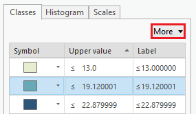
- On the bottom half of the symbology pane, click the More drop-down button and select Formal all symbols.
- Use the ‘Outline Color’ Click Properties. Use the ‘Outline Color:’ drop-down menu to select No No Color.
- Click Apply.Symbolize the Subbasin layer using the same symbology as you used in the Lab1 map document Apply.
Now you will calculate the water storage capacity of the top 1 m of soil within the Buffalo-San Jacinto subbasin.
- Open the Soils layer attribute table.
- Calculate statistics for the Available Water Storage 0-100 cm – Weighted Average field.
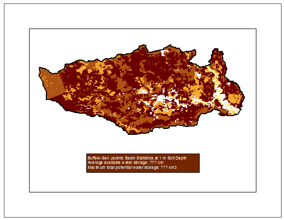
Based on the statistics you have just seen, calculate the answers to the questions listed for the map layout to be turned in on the following pagebelow. Note that, technically, a true calculation of the average available water storage for the subbasin would require factoring in the area of each soil polygon to calculate a weighted average. In this case, just use the statistical mean as it is listed in the ‘Statistics’ window. Similarly, the total water storage for the subbasin would require multiplying the available water storage by the area of each soil polygon and then summing the results. In this case, you may simply multiply the area of the entire subbasin by the statistical mean as it is listed in the ‘Statistics’ window.
As before, create a new map layout and add the statistics using a rectangle text element. When your layout is complete, export it as a PDF.
TO BE TURNED IN: An 8.5 x 11 map document showing the soils clipped to the Buffalo-San Jacinto subbasin and a text box containing the answers to the following questions:
- What is the average available water storage (cm) in the Buffalo-San Jacinto subbasin?
- Based on your previous calculation of the area of the subbasin in km2, what volume of water (km3) could potentially be stored in the top 1 m of soil in the Buffalo-San Jacinto subbasin if the soil were fully saturated with water?
Exporting map documents
- To export both your Lab1Hydrology and Lab1Soils map documents, open each of them in turn and click the Share menu and select Export Layout….
- Navigate to your HydrologyLab folder.
- Use the ‘Save as type:’ drop-down menu to select PDF.
- Click Export.
- Print both map PDFs to turn inin the top 1 m of soil in the Buffalo-San Jacinto subbasin if the soil were fully saturated with water?
Deliverables
- Create an 8.5 x 11 layout with the following layers limited to the subbasin:
- Subbasin – hollow outline
- Watersheds – categorical symbology and labeled
- Flowlines – graduated symbology
- Stream gages – point symbol
- Basemap
...
Include a text box in the layout containing the answers to the following questions:
...
- How many HUC-12 catchments are there in the Buffalo-San Jacinto Basin?
...
- What is their average area in km2?
...
- What is the total area of this subbasin in km2?
...
- What is the ratio of the length of the streamlines to the area of the Buffalo-San Jacinto subbasin (called the drainage density) in km-1?
2. Create an 8.5 x 11 layout with the following layers limited to the subbasin:
- Subbasin – hollow outline
- Soils – graduated colors
Include a text box in the layout containing the answers to the following questions:
...
- What is the average available water storage (cm) in the Buffalo-San Jacinto subbasin?
...
- Based on your previous calculation of the area of the subbasin in km2, what volume of water (km3) could potentially be stored in the top 1 m of soil in the Buffalo-San Jacinto subbasin if the soil were fully saturated with water?
...