| Info |
|---|
This guide was created by the staff of the GIS/Data Center at Rice University for the custom course - ESCI 545 Hydrocarbon Systems Analysis - and is to be used for individual educational purposes only. The steps outlined in this guide require access to ArcGIS Pro software and data that is available both online and at Fondren Library. The following text styles are used throughout the guide: Explanatory text appears in a regular font.
Folder and file names are in italics. Names of Programs, Windows, Panes, Views, or Buttons are Capitalized. 'Names of windows or entry fields are in single quotation marks.' "Text to be typed appears in double quotation marks." |
| Info |
|---|
| Info |
|---|
| Course Objective: Use GIS workflows to collate and synthesize datasets to create geologic and play elements maps that will be used in petroleum system and risk analysis of potential opportunities and plays. |
Table of Contents
Getting Started
For more practice navigating the ArcGIS Pro interface, check out our short course: Introduction to ArcGIS Pro
Creating a New Project in ArcGIS Pro
- From the Start menu, launch ArcGIS Pro.
- When ArcGIS Pro opens, under the New Blank Template section, click the Map project template.
- In the 'Create a New Project' window, for Name, type "PlayMapping".
- For Location, click the Browse... button to the right.
- In the 'Select a folder to store the project.' window, click Computer in the left column and click Desktop in the right column and click OK.
- In the 'Create a New Project' Window, click OK.
- Maximize the ArcGIS Pro application window.
Editing the New Map
A map is a project item used to display and work with geographic data in two dimensions. The first step to visualizing any data is creating a new map. The Ribbon runs horizontally across the top of the ArcGIS Pro interface. Tools (buttons) are organized into tabs along the Ribbon.
You will notice that a new Map View opens in the main section of ArcGIS Pro. The panel on the left side of ArcGIS Pro is called the Contents pane. The Contents pane displays the default Map title and automatically adds the Topographic basemap layer to the map.
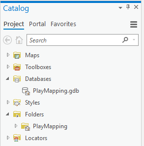
The panel on the right side of ArcGIS Pro is called the Catalog pane. The Maps section is at the top of the Project tab within the Catalog pane.
- In the Catalog pane, click the arrow to expand the Maps section.

Notice that there is a single map there, named Map. Since most projects will have multiple maps, it is a good idea to name your maps with more descriptive titles. - In the Catalog pane, under the Maps section, right-click Map and select Rename.
- Type "GISWorkshop" and hit Enter.
Saving a Project
Any time you create a new project item (such as a map or a layout), spend time adjusting the symbology of your map layers, or are preparing to run a tool, it is a good idea to save your project.
- Above the Ribbon, on the Quick Access toolbar, click the Save button.
Data Management
For more practice with Data Management, check out our short course: Introduction to GIS Data Management
Download Workshop Data
- Click Workshop_Data.zip above to download the tutorial data. Make a note where this file is saved on your personal computer.
- Open your Downloads folder.
- Right-click Workshop_Data.zip and select Extract All....
- In the Extract Compressed (Zipped) Folders window, accept the default location into the Downloads folder.
- Click Extract.
Browsing Existing Data
- In the Catalog pane, click the arrow to expand the Databases section.
- Click the arrow to expand the PlayMapping.gdb geodatabase. You will notice there is no data in the project geodatabase. Over the next few sections, we will transfer and generate data to this project geodatabase.
- In the Catalog pane, click the arrow to expand the Folders section. Again, notice there is no data in the folder, just the default PlayMapping folder created with this project.
Connecting to a Folder
- In the Catalog pane, right-click Folders and select Add Folder Connection.
- Navigate to your personal downloads folder and click on Downloads.
- Click OK.
- In the Catalog pane, expand Downloads and then expand the Workshop_Data folder.
- Your Workshop_Data folder should look like the below image.

- Expand the SpatialJoinData.gdb so you can see the geologic_features_poly feature class.
Importing Data to Project Geodatabase and Project Folder
- In the Catalog pane, click-and-hold the geologic_features_poly geodatabase feature class from the SpatialJoinData.gdb and drag-and-drop it up into the PlayMapping.gdb. A progress bar will appear that reads 'Copying...' Once it is complete, you will see a copy of geologic_features_poly inside the PlayMapping.gdb.
- In the Catalog pane, click-and-hold the HST.jpg from the Workshop_Data folder and drag-and-drop it up into the PlayMapping project folder.
- In the Catalog pane, click-and-hold the IGOR_masterlist excel file from the Workshop_Data folder and drag-and-drop it up into the PlayMapping project folder.
- In the Catalog pane, in the Folders section, right-click on Downloads and select Remove.
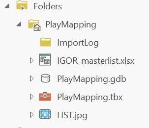
- Your PlayMapping project folder should look like the below image.
Adding Data to a Map
For more practice with Coordinate Systems, check out our short course: Introduction to Coordinate Systems and Projections
- The map takes on the projection of the first data layer added. If a JPG is added first, then the map projection would be undefined (as the projection for a JPG is undefined). To define the map's coordinate system, in the Contents pane on the left, right-click the GISWorkshop map and navigate to Properties > Coordinate Systems > Geographic Coordinate Systems > North America > USA and Territories > NAD 1927.
- Click OK in the Properties window.
- In the Catalog pane, right-click the HST.jpg raster and select Add To Current Map.
- An alternative method of adding data to a map is to click-and-hold the item and drag-and-drop it into the Map View.
Georeferencing
Georeferencing is the process of defining the location of raster data using map coordinates which allows it to be viewed, queried, and analyzed with your other geographic data. For more practice with Georeferencing, check out our short course: Mapping Imagery. For more information on Georefencing in ArcGIS Pro, check out this help resource: Georeferencing
When Georeferencing, as well as later editing we will do in this course, click and hold the mouse scroll wheel to pan across the screen when you are currently in an editing session.
- In the Contents pane, right-click HST.jpg then click Zoom to Layer.
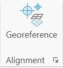
- In the Contents pane, click HST.jpg so that is highlighted in light blue. From the Ribbon, click the Imagery tab and then click the Georeference button.
- Click Add Control Points.

- Left-click the top left corner of the HST JPG. This selects this point on the JPG to georeference. If you need to zoom in and pan around to see the corners of the JPG, you can move the mouse scroll wheel to zoom and click and drag the mouse scroll wheel to pan.
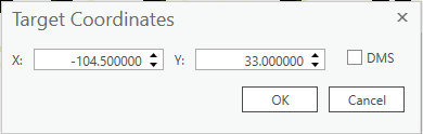
- Right-click anywhere on the map. This opens up a Target Coordinates pop-up box, in which you can manually enter X and Y values.
- Type X : -104.5, Y : 33 and click OK. The x-value is the West coordinate and it is negative because we are in the Western Hemisphere. The y-value is the North coordinate.
- In the Contents pane, right-click HST and click Zoom to Layer.
- Repeat steps 5-8 for the bottom right corner of HST, but type X : -103.5, Y : 32.
- Repeat steps 5-8 for the bottom left corner of HST but type X : -104.5, Y : 32.
- Repeat steps 5-8 for the top right corner but type X : -103.5, Y : 33.
Your georeferenced HST should look like this: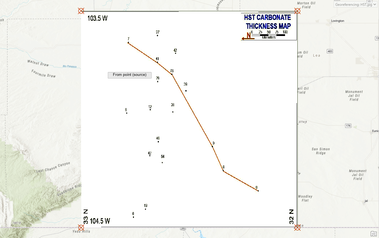
- From the Georeferencing tab, click Save.

- Then click Close Georeference.
- Above the Ribbon, on the Quick Access toolbar, click the Save button.
Digitizing Features
For more practice with Digitizing Features, check out our short course: Creating Vector Data. For more information on digitizing features in ArcGIS Pro, check out this help resource: Creating Features
- In the Catalog pane, expand the Databases section.
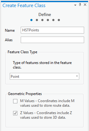
- Right-click PlayMapping.gdb and select New > Feature Class.
- Name it "HSTPoints".
- Under the Feature Class Type drop-down box, select Point.
- Click Next twice.
- In the Spatial Reference section, under the Layers section, select the NAD 1927 projection.
- Click Next twice again.
- Click Finish.
- If the new feature class did not automatically iadd to your map: From the Catalog pane in the Databases section, expand PlayMappping.gdb. Right-click HSTPoints and select Add to Current Map.
- In the Contents pane, right-click HSTPoints and select Attribute Table.
- From the top of the attribute table, next to the Field: section, click the Add button.

- A new Fields view table appears. In the third row of the Field Name column, type "Thickness".
- Change the Data Type to Short Integer by clicking the drop-down box then selecting Short.
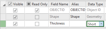
- From the Ribbon, in the Fields tab, click the Save button.
- Close the Fields view table by clicking the X at the top right corner of Fields: HSTPoints.
- From the Ribbon, select the Edit tab.
- From the Edit tab, in the Features group, click Create. A new pane, Create Features, opens on the right side of the screen.

- From the Create Features pane, click HSTPoints and select the Point button (first in list).

- In the Map View, click to add a point on the topmost left point displayed on the HST.jpg.
- In the Attribute Table, a new row has been generated for this newly created point. Click in the Thickness cell for this row and type "7".
- Repeat steps 19 and 20 for all points on HST.jpg.
- From the Edit tab, in the Manage Edits group, click Save.
- Click Yes for the 'Save all edits?' pop-up window.
- In the Edit tab, navigate to the Selection section and click the Clear button to unselect any points.
- Close the Create Features pane.
- Close the Attribute Table.
- Above the Ribbon, on the Quick Access toolbar, click the Save button.
Interpolation
This sections steps through how to interpolate a raster surface from points using a natural neighbor technique. For more practice with Interpolation, check out our short course: Data Interpolation and Extraction. For more information on Natural Neighbor Interpolation in ArcGIS Pro, check out this tool reference: Natural Neighbor (Spatial Analyst)
- From the Ribbon, click the Analysis tab.
- From the Analysis tab, in the Geoprocessing group, click the Tools button. A new pane, Geoprocessing, will appear on the right side of the screen.

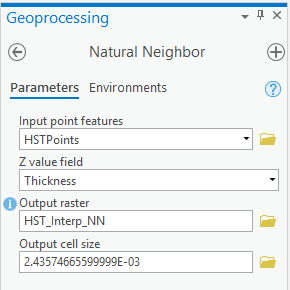
- In the Geoprocessing pane, type "Natural Neighbor" into the 'Find Tools' search bar.
- Select Natural Neighbor (Spatial Analyst Tools).
- Under Input point features, click the drop-down menu and select HSTPoints.
- Under Z value field, choose Thickness.
- Under Output raster, change the name to HST_Interp_NN.
- When your Geoprocessing pane looks like this, click Run.
Your output raster should look like this:
- Above the Ribbon, on the Quick Access toolbar, click the Save button.
Symbology
For more practice with Symbology, check out our short course: Introduction to ArcGIS Pro. For more information on Symbology in ArcGIS Pro, check out this help resource: Symbology
- In the Contents pane, right-click HST_Interp_NN and select Symbology. A new pane, Symbology, will open up on the right side of the screen. From here you can change the symbology settings, which affects how the HST_Interp_NN raster is displayed on the map. Stretched symbology displays continuous raster cell values across a gradual ramp of colors. Classified symbology displays thematic rasters by grouping cell values into classes.
- In the Symbology pane, choose Classify from the Primary symbology drop down menu. To change the number or classes, use the drop-down box under Classes. To manually alter the class intervals, double-click the upper values box you would like to edit and enter the new values. To change the color, use the drop-down options under Color Scheme.
- In the Symbology pane, choose Stretch from the Primary symbology drop down menu. To change the color, use the drop-down options under Color Scheme.
- Above the Ribbon, on the Quick Access toolbar, click the Save button.
Contour
This section steps through how to generate contour lines by joining points with the same elevation from a raster dataset. For more information on the Contour tool in ArcGIS Pro, check out this tool reference: Contour
- From the Ribbon, click the Analysis tab.
- From the Analysis tab, in the Geoprocessing group, click the Tools button. The Geoprocessing pane will appear on the right side of the screen.
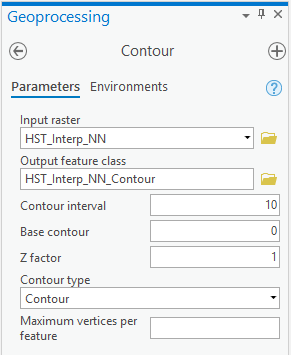
- In the Geoprocessing pane, type Contour.
- Select Contour (Spatial Analyst Tools).
- From the Input raster drop-down menu, select HST_Interp_NN.
- Under Output polyline features, type "HST_Interp_NN_Contour".
- Under Contour interval type "10".
- Leave the Base contour as 0.
- Leave the Z factor as 1. If you were using a different thickness than feet, you would want to input the conversion factor here.
- When your Geoprocessing panel looks like this, click Run.
- Above the Ribbon, on the Quick Access toolbar, click the Save button.
Importing Excel Data
For more practice with displaying XY data, check out our short course: Mapping Locations Using XY Coordinates. For more information on working with Excel in ArcGIS Pro, check out this help resource: Work with Excel in ArcGIS Pro
- From the Ribbon, click the Analysis tab.
- From the Analysis tab, in the Geoprocessing group, click the Tools button. The Geoprocessing pane will appear on the right side of the screen.
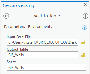
- In the Geoprocessing pane, type Excel to Table.
- Select Excel to Table (Conversion Tools).
- For Input Excel File, click the Browse button.
- On the left side of the Browse window, click Folders.
- On the right side of the Browse window, double click the PlayMapping folder and choose IGOR_masterlist
- Under Output Table, name the table GIS_Wells.
- From the Sheet drop down, choose the GIS_Wells sheet. This ensures that the GIS_Wells sheet will be the data converted from an excel table to a geodatabase table.
- When your Geoprocessing pane looks like this, click Run.
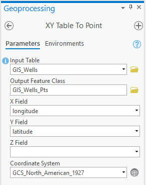
- In the Contents pane, right-click the GIS_Wells table and select Display XY Data.
- Name the layer "GIS_Wells_Pts".
- Check that the X Field states "longitude" and the Y Field states "latitude".
- For Coordinate System, use the dropdown menu to select Current Map [GISWorkshop]. The coordinate system should now be GCS_North_American_1927.
- When your Geoprocessing pane looks like this, click Run.
- In the Contents pane, rick-click on GIS_Wells_Pts and select Zoom to Layer.
- In the Contents pane, right-click GIS_Wells_Pts and select Label.
- Right-click GIS_Wells_Pts and select Label Properties. A new pane, Label Class, will open on the right side of the screen.
- Under the Expression box, clear the current input.
- Under the Fields box, double click api_number. The Expression box should now read $feature.api_number.
- When your Label Class pane looks like this, click Apply.

- Above the Ribbon, on the Quick Access toolbar, click the Save button.
Spatial Join
This section steps through how to joins attributes from one feature to another based on a spatial relationship. For more practice with Spatial Joins, check out our short course: Introduction to Geoprocessing. For more information on Spatial Join in ArcGIS Pro, check out this tool reference: Spatial Join
- In the Catalog pane, expand PlayMapping.gdb.
- Right-click on geologic_features_poly and select Add to Current Map.
- In the Contents pane, right-click on geologic_features_poly and select Symbology.
- From the Symbology pane, use the dropdown menu to select Unique Values.
- Change the Field 1 selection to FEATURE.
- From the Color Scheme drop-down, select the color scheme that you would like.
- From the Ribbon, click the Analysis tab.
- From the Analysis tab, in the Geoprocessing group, click the Tools button. The Geoprocessing pane will appear on the right side of the screen.
- In the Geoprocessing pane, type Spatial Join.
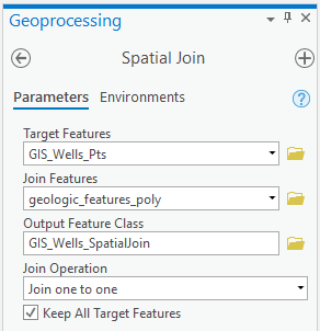
- Select Spatial Join (Analysis Tools).
- Under Target Features, select GIS_Wells_Pts.
- Under Join Features, select geologic_features_poly.
- Rename the Output Feature Class as GIS_Wells_SpatialJoin.
- Retain the default setting of Join_one_to_one for the Join Operation.
- Retain all other default settings.
- When your Geoprocessing pane looks like this, click Run.
- In the Contents pane, right-click on GIS_Wells_Pts and select Remove.
- In the Contents pane, double-click on GIS_Wells_SpatialJoin and rename it GIS_Wells.
- Above the Ribbon, on the Quick Access toolbar, click the Save button.