Page History

...

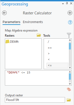
1. In the Raster Calculator tool, delete the previous expression "DEMSubbasin" * 3.281.
2. In the list of 'Rasters’, double-click the DEMft layer.
3. In the list of 'Tools', double-click the <= sybmol symbol.
4. In the equation box, type “15”.
5. For ‘Output raster’, rename the raster from demft_raster to “Flood15ft”.
6. Ensure your Geoprocessing pane appears as shown below and clickRun.
   
   
   
   
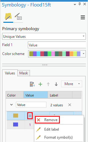
7. In the Contents pane, right-click the Flood15ft layer and selectSymbology.
8. In the Symbology pane, right-click the 0 value and clickRemove.
   
   
   
   
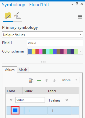
9. Click the rectangle symbol to the left of the 1 value and select Blue.
   
   
   
   

...

Now you will create a new map document from the one you are currently using.

1. Click On the ribbon, click the Insert menu tab and select click the New Map button.
2. Double-click “Map1” in the contents pane and type “Lab2Topo” as name. Click SaveIn the Contents pane, rename the map “Lab2Topo”.
3. Expand Databases in the Catalog pane. Click HydrologyLab.gdb.
4. Drag the DEMft and Watersheds_Stateplane layers into the map display.
5. Turn off the Watersheds_Stateplane layer.
6. Right-click DEMft layer and click the Symbology.
7. Scroll down the ‘Color Ramp’ drop-down menu and select the rainbow ramp.
   
   

...

In addition to raster DEM data, it is sometimes useful to be able to represent elevation using vector contour lines. Contour lines at any regular intervals or discrete values can be created from DEM data.

1. Open Return to the Geoprocessing pane by clicking Tools from Analysis tab.
2. At the top left of the Geoprocessing pane, click the Back button.
3. In the search box, type "Contour".
4. Click the Contour (Spatial Analyst Tools) In the Spatial Analyst Tools toolbox, click the Surface toolset then click the Contour tool.
5. For ‘Input raster’, select the DEMft layer.
6. For the ‘Output polyline features’, rename the feature class from “Contour“Contour_DEMft1” to “Contours10ft”DEMft1” to “Contours10ft”.
7. For ‘Contour interval’, type “10” “10”.

The base contour is the lowest contour that will be shown. Since the lowest elevation is -26 ft, you will set your base contour to -20 ft.

...

1. For ‘Z factor’, leave the default value of 1.
2. Ensure your ‘Contour’ window appears as shown below and click Run.
   
   
   
   
3. Turn off the DEMft layer to better see the contours.
4. Right-click the Contours10ft layer. Click Symbology.
5. Use the drop-down menu at the top to select Unique values.
6. Use the ‘Value Field’ drop-down menu to select the Contour field.
7. Use the ‘Color Ramp’ drop-down menu. Check Show All and select one of the few graduated color ramps as shown below. 
   
   
   
   
8. Now you can tell which contours are highest and lowest.
9. Turn off and collapse the Contours10ft layer.
10. Turn back on the DEMft layer.

Generating a hillshade

...

1. Open Geoprocessing pane by clicking Tools from Analysis tab.
2. In the Surface toolset, double-click the Hillshade tool.
3. For ‘Input raster’, select the DEMft layer.
4. For ‘Output raster’, rename the raster from “HillSha“HillSha_DEMf1” to “Hillshade”DEMf1” to “Hillshade”.

The azimuth and altitude refer to sun angles. For now, you will stick with the default values.

...

1. In the Contents pane, drag the Hillshade layer beneath the DEMft layer.
2. In the DEMft layer, in the feature-dependent Appearance tab, in the Effects group, slide the transparency to 60%.

Now the gradual changes in elevation are apparent from the coloring and are complimented by a realistic display of the terrain created with the hillshade.

1. Turn on the Watersheds_StatePlane layer.
2. Symbolize the Watersheds_StatePlane layer with a hollow fill and thick black outline.

...

1. Click the Catalog tab.
2. In the HydrologyLab geodatabase, drag the Flowlines feature class into the Map Display.
3. In the Contents pane, drag the Flowlines layer above the DEMft layer, but beneath the Watersheds_StatePlane layer.
4. Symbolize the Flowlines layer with a thin blue line.
5. Save your map document project.

FOR MAP LAYOUT TO BE TURNED IN

...

1. Open Geoprocessing pane by clicking Tools from Analysis tab.
2. In the Spatial Analyst Tools toolbox, double-click the Zonal toolset then click Zonal Statistics as Table tool.
3. For ‘Input raster or feature zone data’, use the drop-down menu to select the Watersheds_StatePlane layer.
4. Use the ‘Zone field’ drop-down menu to select the ‘HU‘HU_10_NAME’ NAME’ field.
5. For ‘Input value raster, select the DEMft layer.
6. For ‘Output table’, rename the table from “ZonalSt“ZonalSt_Watersh1” to “WatershedElevation”Watersh1” to “WatershedElevation”.
7. Ensure your ‘Zonal Statistics as Table’ window appears as shown and click Run.
   
   
   
   
8. In the Contents pane, right-click the WatershedElevation table and select Open.

This table tells you the statistics regarding all the elevation values within each watershed zone.

...

If you save this table inside your file geodatabase, you will not be able to open it outside of ArcGIS, so you will instead save it as a text file outside of your file geodatabase.

1. Save the table within the HydrologyLab folder.
2. For ‘Name’, name as “WatershedElevation”.
3. In the ‘Table to Excel’ window, click Run.
4. Close the Table.

...

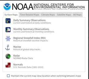
1. On the Surface Maps tab, click Normals.
   
   
   
   
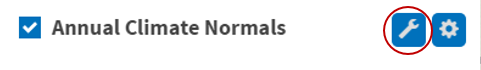
2. In the left sidebar, on the Layers tab, uncheck Daily Climate Normals, and check Annual Climate Normals.
3. To the right of Annual Climate Normals, click the Map Tools button.
   
   
   
   
4. In the new ‘ANNUAL CLIMATE NORMALS TOOLS’ window, click Location.
5. Use the drop-down menu to select USGS HUC.
6. Use the ‘Select a HUC type’ drop-down menu to select Subregions (4-digit).
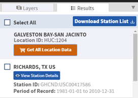
7. Use the ‘Select a HUC’ drop-down menu to select Galveston Bay-San Jacinto.
   
   
   
   
8. Click Zoom to location.
9. The left sidebar switches to the Results tab. Click Get All Location Data.
   
   
   
   
10. For Step 1, select CSV for the output format and click CONTINUE.
    
    
    
11. For ‘Station Detail & Data Flag Options’, check Station name, Geographic location, and Include data flags to include those variables the data table.
    
    
    
    
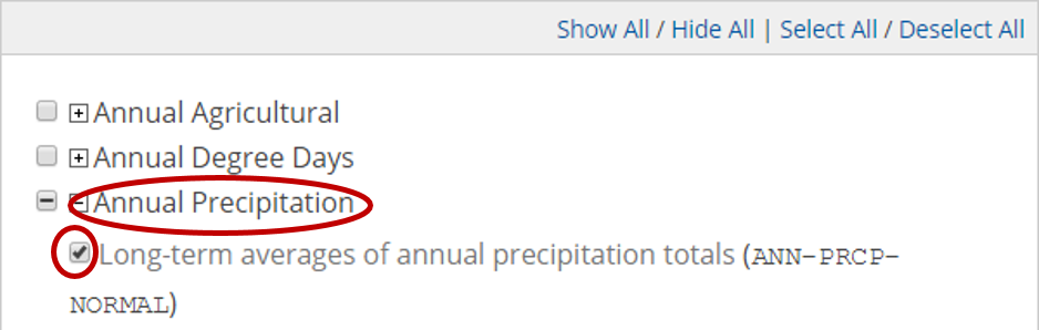
12. For ‘Select data types for custom output’, click the Annual Precipitation category to expand it.
13. Check Long-term averages of annual precipitation totals (ANN-PRCP-NORMAL).
    
    
    
    
14. At the bottom of the window, click CONTINUE.
15. Type your email address twice and click SUBMIT ORDER.

...

1. Rename “ANN-PRCP-NORMAL” to “ANNPRCPHI”, for annual precipitation in hundredths of inches.
2. Along the top of the worksheet, drag across the column letters to select columns A through H.
3. Copy the columns. Along the bottom of the worksheet, click the "plus" icon to create a new sheet. In the A1 cell, paste your previously copied columns. 
4. Delete the previous sheet. 
5. Along the top of the worksheet, drag across the column letters to select columns A through H.
6. Hover your mouse between columns G and H until the cursor changes to two outward facing arrows and double-click to auto-size the column widths.
7. At the bottom left of the worksheet, rename the worksheet “PrecipStations”.
8. Click the File menu and select Save As.
9. Navigate to your HydrologyLab folder.
10. For ‘File name:’, type PrecipStations.
11. Use the ‘Save as type:’ drop-down menu to select Excel 97-2003 Workbook.
12. Click Save.
13. Close Excel.

Displaying XY data

...

1. Return to ArcGIS Pro.
2. Click the Insert menu and select New Map.
3. Click “Map1” in the contents pane to rename it as “Lab2Precip”. Click Save.
4. Drag Watersheds_Stateplane onto the map display.
5. Click the Geoprocessing tab and search for ‘Excel to Table’.
6. For the Input Excel File, selectPrecipStations. Rename the output table PrecipStations.
7. Click Run.
8. In the Contents pane, right-click the PrecipStations table and select Display XY Data.
9. For ‘X Field:’, select the LONGITUDE field.
10. For ‘Y Field:’, select the LATITUDE field.
11. Click the Atlas to the right of the Spatial Reference box.

...

Now you will calculate precipitation for each watershed using a different interpolation method.

1. Turn off the ThiessenWatershedIntersect layer.
2. Right-click the Watersheds_StatePlane layer and select Zoom to Layer.
3. Open Toolbox.
4. In the Spatial Analyst Tools toolbox, click the Interpolation toolset then the Spline tool.
5. On the top of the window, click the Environments tab.
6. For Extent, use the drop-down menu to select Current Display Extent.
7. Use the ‘Mask’ drop-down menu to select the Watersheds_StatePlane layer.
8. Go back to Parameters. For ‘Input point features’, drag in the PrecipStations_StatePlane layer.
9. Use the ‘Z value field’ drop-down menu to select the ANNPRCPHI field that contains the values you wish to interpolate.
10. For ‘Output raster’, rename the exported raster from “Spline_Preci1” to “AnnPrecip”“AnnPrecip”.
11. Use the ‘Spline type’ drop-down menu to select TENSION.
12.  Ensure your ‘Spline’ window Geoprocessing pane appears as shown below, and click Run.
    
    
    
    

The result is a solid surface estimating the rainfall at each cell, based on the data collected at each rain gage. Turn the Thiessen polygons back on to give them a hollow fill. Symbolize the rain gages as you desire.

...