TABLE OF CONTENTS

This course will teach you how to download, evaluate, and prepare GIS data from public online sources and set up a project in ArcGIS Pro.

Obtaining Tutorial Data

COHGIS Open Data Portal

The COHGIS (City of Houston GIS) Open Data Portal website provides over 100 data sets including administrative boundaries, amenity locations, transportation routes, crime, and flooding. 

1. Using a web browser, search for "houston gis data" and select the result as shown below or or go directly to: https://cohgis-mycity.opendata.arcgis.com/.
   
   

Whenever you see a URL that ends in opendata.arcgis.com, you will know that you are visiting a standard ArcGIS Open Data portal.

1. In the 'Search for Data' box, type "historic sites" and press Enter.
2. Click the second option for COH HISTORIC SITES/LANDMARKS, as shown below.
   
   

1. In the middle right of the page, click Download > Shapefile.
   
   

H-GAC GIS Datasets

The Houston-Galveston Area Council (H-GAC) is the 13-county Metropolitan Planning Organization (MPO) for the Houston region. Federal legislation requires that an MPO be designated for each urbanized area with a population greater than 50,000 people (as established by the U.S. Census Bureau) in order to conduct long-range metropolitan transportation planning and be eligible for Federal funding for transportation projects. Their mission to carry out metropolitan transportation planning means that MPOs are a great source of data on topics such as demographics, employment, land use, transportation, and environmental conditions and most of these topics are well-suited towards GIS analysis.

Most of the data provided on the H-GAC portal is not originally created by the H-GAC, but rather is either aggregated from multiple municipalities up to the 13-country region, or clipped from the country or state down to the 13-county region.

1. Using a web browser, search for "h-gac gis" and select the result as shown below or go directly to: http://www.h-gac.com/gis-applications-and-data/datasets.aspx
   
   
   
   
2. Under the 'Dataset Categories' section, click the Hydrologic button to filter the results by subject.
   
   
3. Under the 'Datasets' section, click Major Rivers.
   
   
4. Click Download Dataset in the pop-up window.
5. Click the blue Download button in the top right corner of the new window.

IPUMS NHGIS Datasets

The National Historical Geographic Information System (NHGIS) provides free online access to summary statistics and GIS boundary files for U.S. censuses and other nationwide surveys from 1790 through the present. NHGIS datasets are large and require additional processing steps for use in ArcGIS Pro. Therefore, a sample of this data will be provided later in this tutorial. If you are in interested in using NHGIS data for your project, please visit the GDC lab or use this link to book an appointment at the GDC for further assistance: https://library.rice.edu/services/gis-assistance

Preparing the Downloaded Data for ArcGIS Pro

Once you have downloaded the historic sites from COHGIS and the major rivers data from H-GAC, you will be able to find the data files in your Downloads folder. You will see that all the files are zipped, meaning they contain compressed files of data within them (you can tell a file is zipped when the file type column reads “Compressed (zipped) Folder”). You will need to unzip the folders to be able to see the data inside them. 

1. On the Desktop, click the File Explorer icon located on the Windows Taskbar on the bottom left corner of the screen. 
2. Navigate to the Downloads folder.
3. Ensure that you see the following zipped folders in your Downloads folder.
   
4. Select both folders.
5. Right-click any of the selected folders and select 7-Zip > Extract Here. Your data is now in its decompressed format and ready to be brought into ArcGIS Pro.
   
   

Creating a New Project in ArcGIS Pro

1. From the Windows Taskbar, click the blue globe icon to launch ArcGIS Pro.
   
   
   
   
2. When ArcGIS Pro opens, under the 'Create a new project' section on the right side of the screen, click the Blank project template.
   
   
   
   
3. In the 'Create a New Project' window, for the 'Name' input, type "Intro_Part2".
4. For 'Location', click the yellow Browse... button to the right.
5. In the 'Select a folder to store the project.' window, click Computer in the left column and click Desktop in the right column and click OK.
   
   
   
   
6. In the 'Create a New Project' Window, click OK.
7. Maximize the ArcGIS Pro application window.

Managing GIS Data

1. In the Catalog pane, under the Folders section, click the arrow to expand Folders > Intro_Part2 > Intro_Part2.gdb. You will notice there is no data in the geodatabase. Over the next few steps, we will import the data we downloaded online from the Downloads folder to our Project Geodatabase.

Connecting to a folder

1. In the Catalog pane, right-click Folders and select Add Folder Connection.
2. In the left column click This PC. In the right column, click Downloads and click OK.
3. In the Catalog pane, expand Downloads.
4. Fully expand all folders and geodatabases in the Downloads folder.
5. We will repeat the above process to connect to a folder containing a sample of NHGIS data. In the Catalog pane, right-click Folders and select Add Folder Connection.
6. In the left column click This PC. In the right column, click gisdata (\\file-rnas.rice.edu)(R) > Short_Courses_HIST207 > HIST207_GDC2 > NHGIS_Data and click OK.
7. In the Catalog pane, expand NHGIS_Data.
8. Your 'Folders' directory should look like the below.
   
   

Importing and Exporting Data in the Project Geodatabase

For this tutorial, we are working with vector data which is a spatial data format that uses points, lines, and polygons to represent real features on the earth's surface. Vector data is ideal for discrete themes with definite boundaries. A Feature Class is a vector storage data format that represents a homogeneous collection of common features. There are two types of Feature Classes: a Shapefile feature class and a Geodatabase feature class. A Shapefile feature class is an open source format. Its file extension is .shp and its icon is green. A Geodatabase feature class is an Esri proprietary format. A Geodatabase feature class must be stored inside a Geodatabase (.gdb) and its icon is white. To better organize our project, we will import the data we downloaded and the NHGIS sample data into our Project Geodatabase.

1. In the Catalog pane, click the US_tract_1980_Harris_County geodatabase feature class located in the NHGIS folder and drag-and-drop it up into the Intro_Part2.gdb. A progress bar will appear that reads 'Copying...' Once it is complete, you will see a copy of US_tract_1980_Harris_County inside the Intro_Part2.gdb as shown below.
   
   
   
   
2. Repeat the above step to drag-and-dropMajor_Rivers from the Major_Rivers.gdb into the Intro_Part2.gdb. 
3. COH_HISTORIC_SITESLANDMARKS is a Shapefile feature class, so it requires a different method to be imported into the Project Geodatabase. In the Catalog pane, right-click on COH_HISTORIC_SITESLANDMARKS.shp and selectExport > Feature class(es) to geodatabase.
   
   
   
   
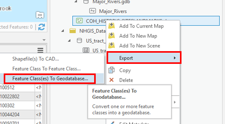
4. Accept default settings as shown below and clickRun. 
   
   
   
   
5. Right-click on Intro_Part2.gdb and selectRefresh. 
   
   
   
   
6. Your Project Geodatabase should now contain three Geodatabase feature classes: COH_HISTORIC_SITESLANDMARKS, Major_Rivers, and US_tract_1980_Harris_County.
   
   
7. In the Catalog pane, in the Folders section, right-click on Downloads and selectRemove.
   
   
8. Repeat Step 7 to remove the connection to the NHGIS folder.

Bonus: Symbolizing Layers By Attributes

Symbolizing Layers By Quantity

1. In the Contents pane, right-click the Census_2010_By_SuperNeighborhood layer name and selectSymbology.

Use the primary 'Symbology' drop-down menu to select Graduated Colors.

Use the 'Field' drop-down menu to scroll down sixth from the bottom and select the SUM_Vacant field. This field stores the number of vacant housing units within each neighborhood.

The map view now displays a choropleth map, where the darker colors represent higher numbers of vacant housing units. In studying the map, it appears as if the most vacant housing is in southwest Houston outside the Loop. While this is true according to raw counts per neighborhood, there could be differences in the neighborhoods that are unaccounted for in this symbology. Now you will try normalizing by the area of the neighborhood.

1. Use the 'Normalization' drop-down menu to scroll to the bottom and select the last Shape_Area field.

As discussed in the Introduction to GIS Data Management course, the projection of the census layer is WGS 1984. Therefore, the layer is unprojected and the coordinates are stored in angular units of decimal degrees. Therefore, the Shape_area field is displaying square decimal degrees and the map is displaying number of vacant housing units per square decimal degree. This is a somewhat incomprehesible unit, however, the values are still proportional to how they would be in a different unit and the relative coloring on the map remains correct. If you wanted to make a map that displays vacant housing units per square mile, then you would add a new field to the attribute table and use the calculate 

projecting is further covered in the Introduction to Coordinate Systems and Projections course.

Notice that according to the density of vacant housing units, the greatest amount of vacant housing units appear to be both inside and outside the loop along 59.

1. Use the 'Normalization' drop-down menu to select the SUM_HU100 field.

The map is now displaying the number of vacant housing units divided by the total number of housing units, or the percent vacant housing units. While all three methods of symbolizing the vacant housing units are techically corect This is probably the most common

1. On the lower half of the Symbology pane, click the Histogram tab.

----------------------------------------------------------------------

Discuss and test classification methods.

----------------------------------------------------------------------

1. Use the 'Method" drop-down menu to selectEqual Interval.

Use the 'Method" drop-down menu to selectQuantile.

----------------------------------------------------------------------

Discuss and test number of classes.

----------------------------------------------------------------------

1. Use the 'Classes' drop-down menu to select20.

Use the 'Classes' drop-down menu to select4.

----------------------------------------------------------------------

Discuss and test color schemes.

----------------------------------------------------------------------

Adding Layer Transparency

1. Ensure that the Census_2010_By_SuperNeighborhood layer is selected.

In the ribbon, click the Feature Layer contextual Appearance tab.

In the Effects group, slide the Layer Transparency slider or type "50" and hitEnter.

Symbolizing Layers By Category

1. Use the primary 'Symbology' drop-down menu to selectUnique Values.

Use the 'Field 1' drop-down menu to selectName.

1. In the Contents pane, collapse the Census_2010_By_Superneighborhood symbology.